Using Excel to automatically flag unusual transactions

Q. I receive accounts payable exports each month and spend too much time sorting, filtering, and scanning transactions to find items that may require follow–up. Can Excel automatically identify unusual transactions and create a report containing only the exceptions?

A. The answer is yes. Exception reporting is one of the most practical ways accountants can use Excel because it directs attention to the relatively small number of transactions that may require additional review. Many accounting systems include standard reports, but accountants still frequently export transaction data to Excel when they need to apply company-specific review criteria, combine several tests, or analyze information received from a client. By adding a few formulas to an accounts payable export and using Excel’s FILTER function, users can create a reusable report that automatically displays only the transactions meeting one or more exception rules.

I used Excel for Microsoft 365 for PCs to create this example. Other Excel versions may work differently. The FILTER and LET functions require a version of Excel that supports dynamic arrays. You can download the Excel file used for this walkthrough and view a video demonstration at the end of this article.

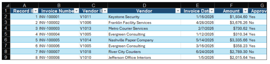
The accompanying workbook contains 300 sample transactions on the AP Export worksheet. The original export includes Record ID, Invoice Number, Vendor ID, Vendor, Invoice Date, Amount, Approved, Approver, Purchase Order, Department, and Payment Terms. Begin by selecting any cell in the data. From the ribbon, select Insert, then Table. Confirm that My table has headers is selected and click OK. Select the newly created table, choose Table Design, and enter Invoices in the Table Name box. Using an Excel table allows formulas to fill down automatically and ensures the data range expands as new rows are added. The following screenshot shows a portion of the sample accounts payable export.

Next, add six columns to the right of the original data and label them High-Dollar Unapproved, Missing PO, Missing Vendor ID, Duplicate Invoice, Weekend Posting, and Exception Status. Each of the first five columns performs a separate exception test. The final column combines the results so the FILTER function can return every transaction with at least one exception.

The first exception test identifies invoices above a selected dollar threshold that have not been approved. In the example workbook, the threshold of 10,000 is entered in cell B3 of the Dashboard worksheet (described later in this column). Place your cursor in cell L2 of the AP Export worksheet, the first data cell under High-Dollar Unapproved, and enter:

=IF(AND(F2>Dashboard!$B$3,G2=”No”),”Yes”,””)

The formula returns Yes only when both conditions are met. Because the data is stored in an Excel table, Excel automatically copies the formula through the remaining rows.

The next two tests identify incomplete transaction data. In cell M2 under Missing PO, enter:

=IF(I2=””,”Yes”,””)

In cell N2 under Missing Vendor ID, enter:

=IF(C2=””,”Yes”,””)

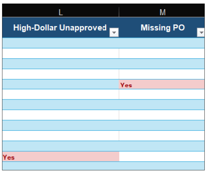
These formulas return Yes when the corresponding field is blank. Missing purchase orders may indicate that established purchasing procedures were not followed, while missing vendor IDs may result from incomplete master data or import problems. The following screenshot shows the exception-test columns for missing data.

Duplicate invoice numbers are another common accounts payable concern. In cell O2 under Duplicate Invoice, enter:

=IF(COUNTIF($B$2:$B$301,B2)>1,”Yes”,””)

COUNTIF compares the invoice number in the current row with the entire Invoice Number range. If the invoice number appears more than once, the formula returns Yes. A duplicate does not necessarily mean that an invoice was paid twice, but it provides a useful starting point for additional investigation.

The final test identifies invoices dated on a Saturday or Sunday. In cell P2 under Weekend Posting, enter:

=IF(WEEKDAY(E2,2)>5,”Yes”,””)

Using 2 as the second argument instructs Excel to number Monday as 1 and Sunday as 7. Therefore, values greater than 5 represent weekend dates. Weekend transactions may be valid, but some organizations include them in journal entry or disbursement reviews because they occur outside the normal business week.

Now combine the five tests in the Exception Status column. The example workbook uses LET to assign short names to each condition and TEXTJOIN to combine all applicable descriptions. In cell Q2, enter:

=LET(HighAmt,L2=”Yes”,MissingPO,M2=”Yes”,DupInv,O2=”Yes”,MissingVendor,N2=”Yes”,WeekendPost,P2=”Yes”,TEXTJOIN(“; “,TRUE,IF(HighAmt,”High-dollar unapproved”,””),IF(MissingPO,”Missing PO”,””),IF(DupInv,”Duplicate invoice”,””),IF(MissingVendor,”Missing vendor ID”,””),IF(WeekendPost,”Weekend posting”,””)))

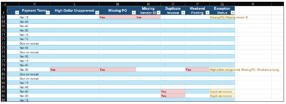
LET makes the longer formula easier to follow by assigning names to each test. TEXTJOIN then lists every exception that applies to the transaction. As a result, one row can display more than one issue, such as “Missing PO; Weekend posting.” The following screenshot shows the completed exception columns.

After the exception tests are complete, go to the Exception Report worksheet. The headings from the source table appear in Row 6. Place your cursor in cell A7 and enter:

=FILTER(‘AP Export’!A2:Q301,’AP Export’!Q2:Q301<>””,”No exceptions found”)

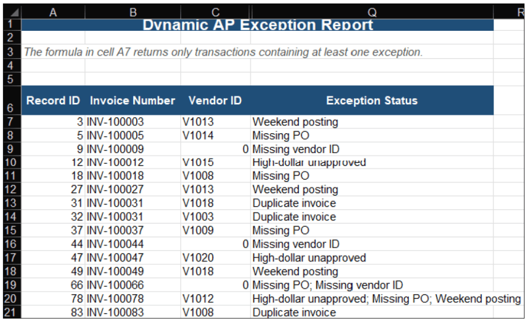
The first argument identifies the range to return. The second argument tells Excel to include only rows in which Exception Status is not blank. The final argument provides a message if no transactions meet the criteria. After pressing Enter, the results spill across the worksheet and display only the transactions requiring review. The following screenshot shows the dynamic exception report.

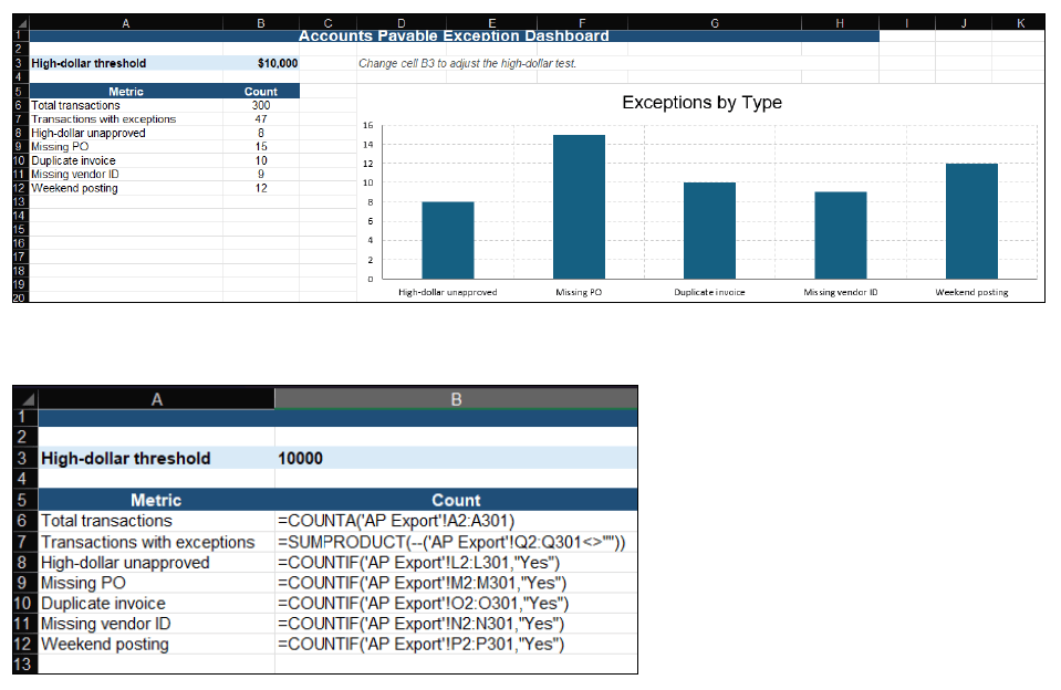
The Dashboard worksheet provides a quick summary. Cell B3 on the Dashboard worksheet contains the adjustable high-dollar threshold. The COUNTA formula in cell B6 counts the total number of transactions. The SUMPRODUCT formula in cell B7 counts the number of transactions containing at least one exception. The COUNTIF formulas (cells B8—B12) calculate the number of high-dollar unapproved invoices, missing purchase orders, duplicate invoice numbers, missing vendor IDs, and weekend postings. A clustered column chart summarizes the five exception types. The following screenshots show the completed dashboard and the formulas used.

Once the workbook is established, it can be reused for future periods. Replace the source transactions in the Invoices table while preserving the column headings and formulas. The formulas, Exception Report, and Dashboard will update when Excel recalculates the workbook. By combining Excel tables, logical formulas, LET, TEXTJOIN, and FILTER, accountants can turn an ordinary transaction export into a focused review tool and spend more time investigating unusual items instead of searching for them.

About the author

Kelly L. Williams, CPA, Ph.D., MBA, is an associate professor of accounting at the Jones College of Business at Middle Tennessee State University.

Submit a question

Do you have technology questions for this column? Or, after reading an answer, do you have a better solution? Send them to jofatech@aicpa.org.