Use Excel dynamic arrays to build a revenue-testing schedule that auto-refreshes

Q. I get a detailed revenue transaction export from the client, and then I get it again, revised, usually after I’ve already filtered, sorted, and documented my selections. I’m tired of reapplying filters and checking whether a formula was copied all the way down. Is there a clean way to build a revenue-testing schedule in Excel that updates when the client file changes?

A. Yes. If you’re using Excel for Microsoft 365 or Excel 2021 or later, you can build the schedule with dynamic array formulas, so Excel returns the workpaper output from a small set of formulas. The advantage is that when the client sends an updated export, you can simply paste it into the same Excel table, and the workpaper will refresh automatically, eliminating the need to re-filter, re-sort, or re-copy formulas.

I used Microsoft Excel 365 for PCs to create this example for applying dynamic array formulas. Other Excel versions may work differently. A video demonstration of creating an interactive revenue-testing schedule is available at the end of this item, and you can download the Excel file I used.

This example produces a distinct list of revenue accounts present in the client’s revenue transaction export and a schedule of individually significant transactions above a threshold, sorted from largest to smallest. An optional step shows how to pull in customer names using XLOOKUP.

First, paste the client’s revenue transaction export into a worksheet. Use a clean sheet and name it Revenue_Data. The export should include the following columns for this example: Date, Invoice, CustomerID, RevenueAccount, and Amount. Click any cell inside the dataset. From the ribbon, select Insert, then Table, and confirm that My table has headers is checked. Click OK. While the table is still selected, go to Table Design within Table Tools, then click Table Name and rename the table tblRevenue.

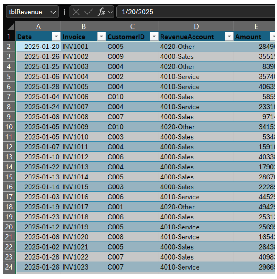
Why does making this into a table matter? An Excel table automatically expands when rows are added or removed. That means your formulas keep pointing to the full export even if the client’s revised file has a different number of rows. The following screenshot shows the revenue transaction export stored as an Excel table named tblRevenue. 

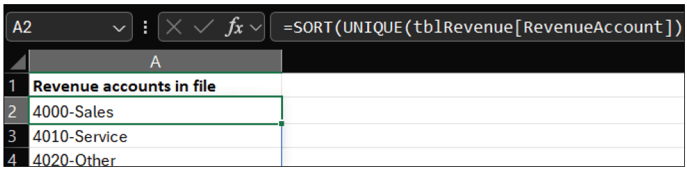
Insert a new worksheet for your workpaper output and name the tab Workpaper. In cell A1, type Revenue accounts in file. In cell A2, enter the formula =SORT(UNIQUE(tblRevenue[RevenueAccount])) and click Enter. This produces a distinct list of revenue accounts and sorts them alphabetically. If the client’s revised export includes a new revenue account, it will appear in the list automatically. See the screenshot below for the Worksheet tab.

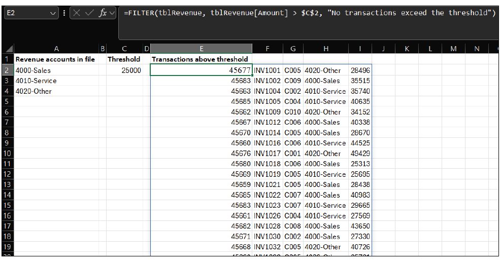
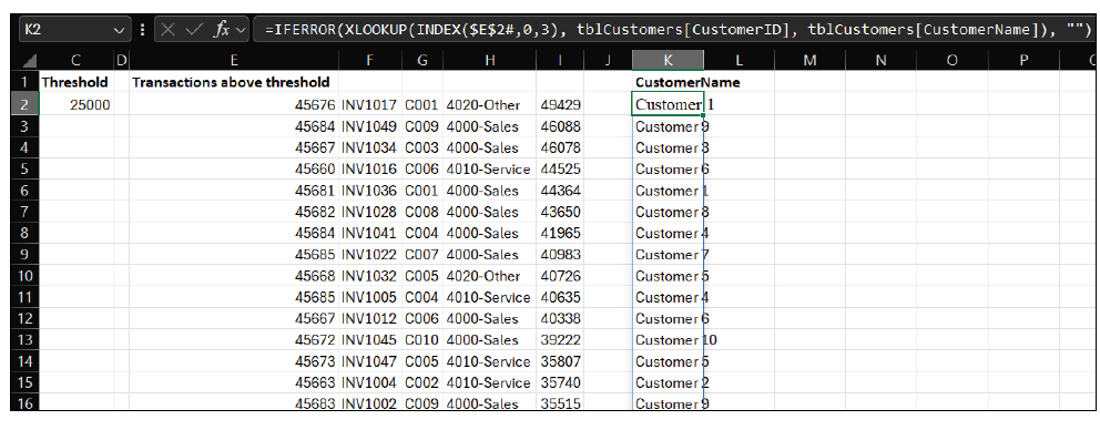
Now, set a threshold so that those transactions can be extracted. In cell C1, enter Threshold. In cell C2, enter the threshold amount. In this example, enter 25000. In cell E1, enter Transactions above threshold. Finally, in cell E2, enter this formula: =FILTER(tblRevenue, tblRevenue[Amount] > $C$2, “No transactions exceed the threshold”). This filter formula returns a spilled schedule, which means one formula produces the full table. If the threshold changes or if the client updates amounts, the output updates automatically. See the screenshot below for this filter formula.

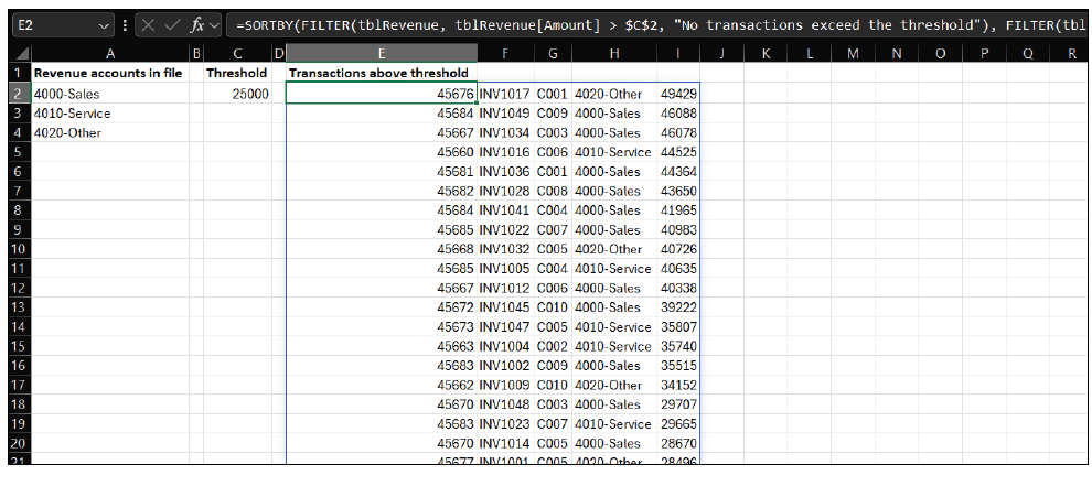
Review work typically starts with the largest items. To sort the extracted schedule from largest to smallest, replace the formula in E2 with this SORTBY version:

=SORTBY(FILTER(tblRevenue, tblRevenue[Amount] > $C$2, “No transactions exceed the threshold”), FILTER(tblRevenue[Amount], tblRevenue[Amount] > $C$2), -1).

This approach avoids manual sorting. The output stays ordered correctly even after a refreshed export is pasted into tblRevenue. See the screenshot for the sorted, filtered version of the transactions.

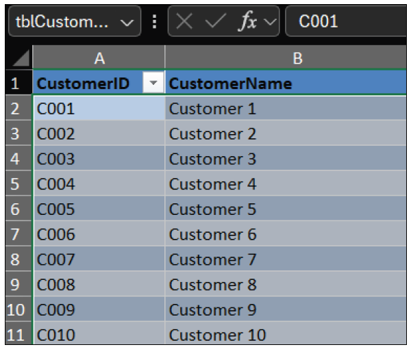
If you want the schedule to show customer names rather than just CustomerIDs, store a customer list in a third Excel tab as a table. Paste your primary customer list into a worksheet named Customer_Master. Convert it to a table by clicking within the data and selecting Insert, Table. Name the table tblCustomers. The minimum columns you need are CustomerID and CustomerName. See a screenshot below of our third tab with the primary customer list.

On the Workpaper sheet, add a column header such as CustomerName next to your spilled schedule. In the first CustomerName cell adjacent to the schedule, enter:

=IFERROR(XLOOKUP(INDEX($E$2#,0,3), tblCustomers[CustomerID], tblCustomers[CustomerName]), “”).

This formula uses the spilled schedule in E2# and retrieves the CustomerID from the third column of the spilled array; it then looks up the customer name. If the customer ID is missing from the primary table, the formula returns a blank (you can swap in “Not found” if you prefer). See the screenshot below for XLOOKUP returning the customer name alongside the spilled schedule.

If you’re still creating threshold schedules manually, you might want to think about using dynamic arrays. By defining the logic just once, Excel will automatically update the schedule whenever the data changes. Revenue testing is an easy place to start, and the same pattern transfers directly to AP, payroll, and journal entry testing.

About the author

Kelly L. Williams, CPA, Ph.D., MBA, is an associate professor of accounting at the Jones College of Business at Middle Tennessee State University.

Submit a question

Do you have technology questions for this column? Or, after reading an answer, do you have a better solution? Send them to jofatech@aicpa.org.