How to use Excel’s AGGREGATE Function

Q. Could you explain how the AGGREGATE function works in Excel?

A. AGGREGATE is possibly the most versatile function in Excel. Think of it as an advanced version of the SUBTOTAL function that offers much more flexibility.

AGGREGATE supports 19 operations, ranging from basic sums and averages to more advanced calculations, such as product and standard deviation. It also offers an additional eight options that allow it to ignore error values in your dataset, ensuring that calculations are not disrupted.

AGGREGATE can exclude hidden rows, which is especially useful for dynamic datasets with filters applied. Unlike SUBTOTAL, the AGGREGATE function can handle other AGGREGATE or SUBTOTAL functions within its calculation. Additional flexibility is demonstrated in this article’s examples.

The AGGREGATE function has two forms: the reference form =AGGREGATE(function_num, options, ref1, [ref2], …) and the array form =AGGREGATE(function_num, options, array, [k]). The arguments are defined as follows:

• function_num, which is required for both forms, is a number between 1 and 19 that specifies the type of calculation to perform. The options include:
  • 1 = AVERAGE
  • 2 = COUNT
  • 4 = MAX
  • 5 = MIN
  • 6 = PRODUCT
  • 7 = STDEV.S
  • 8 = STDEV.P
  • 9 = SUM
  • 10 =VAR.S
  • 11 = VAR.P
  • 12 = MEDIAN
  • 13 = MODE.SNGL
  • 14 = LARGE
  • 15 = SMALL
  • 16 = PERCENTILE.INC
  • 17 = QUARTILE.INC
  • 18 = PERCENTILE.EXC
  • 19 = QUARTILE.EXC
• options, which is required, is a number that determines how the function handles hidden rows, error values, and nested SUBTOTAL or AGGREGATE functions. The options include:
  • 0 or omitted = Ignore nested SUBTOTAL and AGGREGATE functions
  • 1 = Ignore hidden rows, nested SUBTOTAL and AGGREGATE functions
  • 2 = Ignore error values, nested SUBTOTAL and AGGREGATE functions
  • 3 = Ignore hidden rows, error values, nested SUBTOTAL and AGGREGATE functions
  • 4 = Ignore nothing
  • 5 = Ignore hidden rows
  • 6 = Ignore error values
  • 7 = Ignore hidden rows and error values
• Ref1, which is required, is the range of data to apply the function.
• Array, which is required, is the array of values or array formula to apply the function.
• Ref2, which is optional, is for any additional ranges of cells. You can have up to 252 ranges.
• [k], which is optional, is used with function_nums like LARGE, SMALL, PERCENTILE, and others that require a ranking or percentage value.

Don’t worry about which form to use. Excel selects the correct one based on which function_num you chose. Also, don’t worry about trying to remember all the options; Excel will provide drop-down lists with all the choices.

Let’s work on a few examples using the AGGREGATE function. If you would like to follow along, you can download this Excel workbook and watch a video at the end of this article.

See below for a small snippet of the spreadsheet we will use. It contains many account types, account codes, account titles, departments, cost centers, years, months, and budgeted values.

Let’s use both the SUM function and the AGGREGATE function to sum up the budget column, as shown below. In cell H155, enter the AGGREGATE function, with the following syntax: =AGGREGATE(9,3,H2:H151). The 9 instructs Excel to perform a SUM function. The 3 instructs Excel to ignore hidden rows, error values, and nested SUBTOTAL and AGGREGATE functions. H2:H151 is the array or ref1 (it doesn’t matter; Excel will use it properly). See the screenshots below for the formulas and the results.

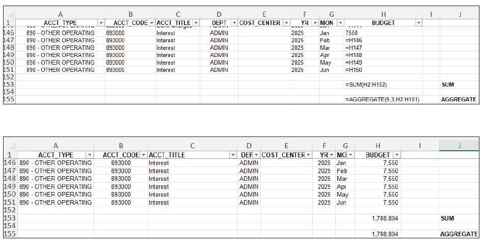
The results are the same for both, so why use AGGREGATE? Because AGGREGATE can do so much more than this! Let’s see how.

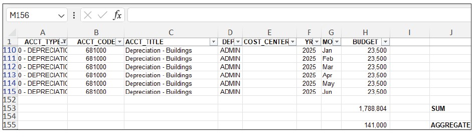
The screenshot below shows what happens when I use the filter on the spreadsheet to show only the account type depreciation. Note that the SUM function still shows the total budget amounts for all account types, but the AGGREGATE function shows only the sum for the depreciation accounts. This is because we chose to ignore hidden rows for our AGGREGATE formula.

In the next screenshot, the spreadsheet contains subtotals based on account type. You can see that the SUM formula adds all the budget values, including all subtotals and the summary total included by the SUBTOTAL formula. This means the SUM formula displays three times the budget’s total. However, the AGGREGATE formula we are using (AGGREGATE(9,3,H2:H151)) calculates the total budget correctly because it instructs Excel to ignore subtotals and aggregate subtotals.

SUBTOTAL also works in the examples above, but that changes when you introduce bad data. An error in a dataset renders SUM and SUBTOTAL unable to complete their calculations, but AGGREGATE can help to sort out the bad data. In the screenshot below, I introduced an error in my budget values. This error has caused the SUM formula to no longer work (SUBTOTAL returns the same error), but because the AGGREGATE formula was instructed to ignore errors, Excel sums the budget numbers while overlooking the error.

We have barely scratched the surface of the AGGREGATE function’s capabilities. With 19 functions and eight options to choose from, users can customize AGGREGATE in 152 ways, and that doesn’t include all the options for employing it. Consider that despite creating only one version of our formula above, we were able to have it successfully work in three scenarios where the SUM formula could not and one where SUBTOTAL also failed to work. Like SUBTOTAL improves upon SUM, AGGREGATE represents an even bigger leap in functionality. How could (or do) you employ AGGREGATE to do your job better?

About the author

Kelly L. Williams, CPA, Ph.D., MBA, is an associate professor of accounting at the Jones College of Business at Middle Tennessee State University.

Submit a question

Do you have technology questions for this column? Or, after reading an answer, do you have a better solution? Send them to jofatech@aicpa.org.