8 ways to calculate depreciation in Excel

Q. Can you show me how to calculate depreciation in Excel using different depreciation methods?

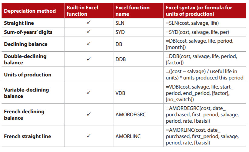
A. There are many ways to calculate depreciation in Excel, and several of the depreciation methods already have a built-in function included in the software. The table below includes all the built-in Excel depreciation methods included in Excel 365, along with the formula for calculating units-of-production depreciation.

These eight depreciation methods are discussed in two sections, each with an accompanying video. The first section explains straight-line, sum-of-years’ digits, declining-balance, and double-declining-balance depreciation. The second section covers the remaining depreciation methods.

For reasons of simplicity and brevity, the depreciation methods demonstrated in this article use only the required arguments. Several of the depreciation functions include optional arguments to allow for more complex facts, such as partial-year depreciation.

You can access the two accompanying videos here and here and a workbook with examples of using the various depreciation methods.

Note that the content that follows is based on Microsoft Excel 365 for PCs. Other versions of Excel may work differently.

SECTION 1

4 depreciation functions and an example

All four depreciation functions covered in this section have three required arguments in common, as follows:

• cost — original cost of the asset;
• salvage — salvage value of the asset (i.e., the book value of the asset after it is fully depreciated); and
• life — useful life of the asset (i.e., how long the asset is estimated to be used in operations).

Those three arguments are the only ones used by the SLN function, which calculates straight-line depreciation.

The SYD function calculates the sum-of-years’ digits depreciation and adds a fourth required argument, per. The syntax is =SYD(cost, salvage, life, per) with per defined as the period to calculate the depreciation. The unit used for the period must be the same as the unit used for the life; e.g., years, months, etc.

The DB function is used for calculating fixed declining-balance depreciation and contains five arguments: cost, salvage, life, period, and month. The first four arguments are required, and the last one is optional. Period is required and represents the period to calculate the depreciation. As with per in the SYD function, the unit used for the period must be the same as the unit used for the life; e.g., years, months, etc. The optional argument, month, refers to the number of months in the first year. If it is left blank, Excel will assume there were 12 months in the first year.

The DDB function is used for calculating double-declining-balance depreciation (or some other factor of declining-balance depreciation) and contains five arguments. The first four (cost, salvage, life, and period) are required and the same as used in the DB function. The fifth argument, factor, is optional and determines by what factor to multiply the rate of depreciation. If it is left blank, Excel will assume the factor is 2 — the straight-line depreciation rate times two, which is double-declining-balance depreciation.

Depreciation example with first four functions

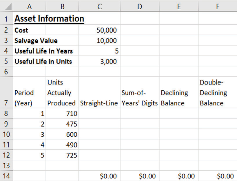
Let’s go through an example using the four methods of depreciation described so far. Assume that our company has an asset with an initial cost of $50,000, a salvage value of $10,000, and a useful life of five years and 3,000 units, as shown in the screenshot below. Our job is to create a depreciation schedule for the asset using all four types of depreciation.

Let’s create the formula for straight-line depreciation in cell C8 (do this on the first tab in the Excel workbook if you are following along). We need to define the cost, salvage, and life arguments for the SLN function. The cost is listed in cell C2 (50,000); salvage is listed in cell C3 (10,000); and life, for this formula, is the life in periods of time and is listed in cell C4 in years (5). Because we are going to copy the formula down so that it calculates the straight-line depreciation for all periods, we will include absolute references ($) in front of the columns and rows of those cells. For this example, the formula we want to enter in cell C8 is =SLN($C$2,$C$3,$C$4). Drag this formula down to populate cells C9 through C12.

The formula for sum-of-years’ digits depreciation is created in cell D8. The arguments to define are cost, salvage, life, and per. Again, the cost is listed in cell C2; salvage is listed in cell C3; life, in periods of time, is listed in cell C4; and per is listed in cell A8. We are going to copy this formula down as we did above with straight-line depreciation, so we will, again, include absolute references ($) in front of the columns and rows of the cells, except for the cell describing the argument per. The reason is that, as we drag the formula down, we want the cell for the period to move down to the next period and so on. For this example, the formula in cell D8 is =SYD($C$2,$C$3,$C$4,A8). Drag this formula down to populate cells D9 through D12.

The formula for declining-balance depreciation is created in cell E8. Cost, salvage, and life are defined and located as with the previous two methods, while period is listed in cell A8. Just as we did with sum-of-years’ digits, include absolute references in front of the columns and rows of the cells, except for the cell describing the argument period. The arguments are exactly the same for declining balance as they were for sum-of-years’ digits for this example. The formula in cell E8 is =DB($C$2,$C$3,$C$4,A8). Drag this formula down to populate cells E9 through E12.

The formula for double-declining-balance depreciation is created in cell F8. The arguments for this example are defined the same as they were for declining balance and sum-of-years’ digits. The formula in cell F8 is =DDB($C$2,$C$3,$C$4,A8). Drag this formula down to populate cells F9 through F12.

If you are following along in the Excel file provided, your worksheet should look like the screenshot below.

The total amount of depreciation taken over the entire life of the asset should equal the depreciable cost (cost minus salvage value). However, accelerated methods of depreciation sometimes do not depreciate to the exact depreciable cost and need to be “plugged.” Of the depreciation methods described above, the accelerated methods of depreciation are declining balance and double-declining balance. You can manually adjust the depreciation expense taken to equal the depreciable cost, or you can include additional formulas to make sure that the total depreciation equals the depreciable cost. If you are interested, these additional formulas are included in the Excel workbook and produce the results shown in the screenshot below.

SECTION 2

4 more depreciation methods and 2 examples

The units-of-production method of depreciation does not have a built-in Excel function but is included here because it is a widely used method of depreciation and can be calculated using Excel. The formula is =((cost − salvage) / useful life in units) * units produced in period. The first two arguments are the same as they were in Section 1, with the other arguments defined as follows.

• useful life in units — the number of units the asset is estimated to produce over the entire life of the asset; and
• units produced this period — the number of units the asset produced this period.

The VDB function calculates double-declining-balance depreciation (or some other factor of declining-balance depreciation) for any period, including partial periods. This function contains seven arguments: cost, salvage, life, start_period, end_period, factor, and no_switch. The first five arguments are required, and the last two are optional. The first three arguments are defined as they were in Section 1. The other arguments are as follows:

• start_period — period to start calculating the depreciation (the unit used for the period must be the same as the unit used for the life; e.g., years, months, etc.);
• end_period — period to end calculating the depreciation (the unit used for the period must be the same as the unit used for the life; e.g., years, months, etc.);
• factor — by what factor to multiply the rate of depreciation (this argument is optional; if it is left blank, Excel will assume the factor is 2, the straight-line depreciation rate times two, which is double-declining-balance depreciation); and
• no_switch — value to specify whether to switch to straight-line depreciation when that calculation is greater than the calculation for declining-balance depreciation (this argument is optional; if it is left blank or the value is FALSE, Excel will switch; if the value is TRUE, Excel will not switch).

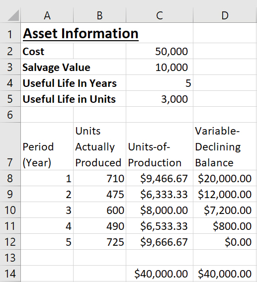
Let’s go through an example using the two methods of depreciation described so far. As with the previous example, assume that our company has an asset with an initial cost of $50,000, a salvage value of $10,000, and a useful life of five years and 3,000 units. This time, we are going to create a depreciation schedule for the asset using the two types of depreciation shown in the screenshot below. To follow along in Excel, access the spreadsheet here and go to the second tab.

Create the formula for units-of-production depreciation in cell C8. The components that are needed are cost, salvage, useful life in units, and units produced this period. The cost is listed in cell C2; salvage is listed in cell C3; useful life in units is listed in cell C5; and units produced this period is listed in cell B8. We want all cells to remain constant, except units produced this period, so we will include absolute references ($) in all cells except this one. The formula in cell C8 is =(($C$2-$C$3)/$C$5)*B8. Drag this formula down to populate cells C9 through C12.

Create the formula for variable-declining-balance depreciation in cell D8. The arguments that need to be defined here are cost, salvage, life, start_period, and end_period. The cost and salvage value are the same as in the previous example, while life, in periods of time, is listed in cell C4; start_period is listed in cell A8; and end_period is listed in cell A8. Because we want the period to extend one entire period, we must include minus 1 in the calculation of the starting period so that it reflects an entire period from start_period to end_period. Include absolute references in front of the columns and rows of the cells, except for the cells describing the arguments start_period and end_period. The formula in cell D8 is =VDB($C$2,$C$3,$C$4,A8-1,A8). Drag this formula down to populate cells D9 through D12.

Your worksheet should look like the one in the screenshot below.

The final two built-in depreciation functions in Excel are AMORDEGRC and AMORLINC. The AMORDEGRC function calculates French declining-balance depreciation, and the AMORLINC function calculates French straight-line depreciation. The two functions contain seven arguments: cost, date_purchased, first_period, salvage, period, rate, and basis. The first six arguments are required, and the last one is optional. The arguments are defined as follows:

• cost — original cost of the asset;
• date_purchased — purchase date of the asset;
• first_period — date of the end of the first period;
• salvage — salvage value of the asset (the book value of the asset after it is fully depreciated);
• period — period to calculate the depreciation;
• rate — rate of depreciation; and
• basis — year basis to use (this argument is optional):
  • 0 or left blank — 360 days (U.S.).
  • 1 — actual.
  • 3 — 365 days.
  • 4 — 360 days (European).

These two functions have the same syntax, but AMORDEGRC contains a depreciation coefficient by which depreciation is accelerated based on the useful life of the asset.

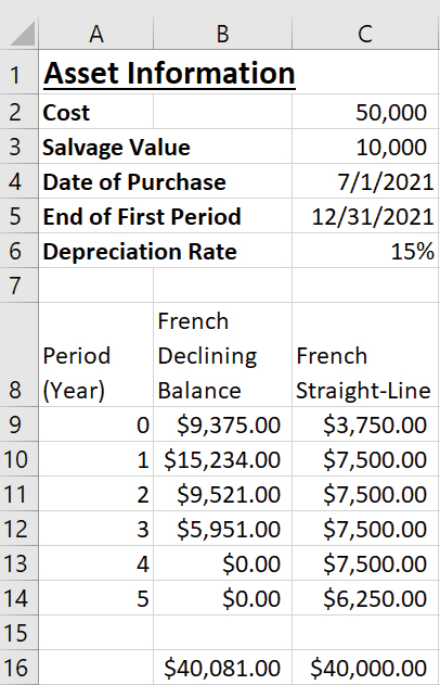
Let’s go through an example using these final two methods of depreciation. Assume that our company has an asset with an initial cost of $50,000, a salvage value of $10,000, a date of purchase of 7/1/2021, an ending of the first period of 12/31/2021, a useful life of five years, and a depreciation rate of 15%, as shown in the screenshot below. Our task is to create another depreciation schedule for the asset using the two French methods. You can follow along with this example on the fourth tab in the Excel spreadsheet.

Create the formula for French declining-balance depreciation in cell B9. The syntax is =AMORDEGRC(cost, date_purchased, first_period, salvage, period, rate, [basis]). The cost is listed in cell C2, date_purchased in cell C4, first_period in cell C5, salvage in cell C3, period in cell A9, and rate in cell C6. These final two depreciation methods begin the depreciation calculation in period 0. Include absolute references in front of the columns and rows of the cells, except for the cell describing the argument period. The formula in cell B9 is =AMORDEGRC($C$2,$C$4,$C$5,$C$3,A9,$C$6). Drag this formula down to populate cells B10 through B14.

The formula for French straight-line depreciation is created in cell C9. The syntax is =AMORDEGRC(cost, date_purchased, first_period, salvage, period, rate, [basis]). All the arguments are defined the same as they were for French declining-balance depreciation. The formula in cell C9 is =AMORLINC($C$2,$C$4,$C$5,$C$3,A9,$C$6). Drag this formula down to populate cells C10 through C14. Your worksheet should now look like the one in the screenshot below.

French declining balance is an accelerated method of depreciation and may need to be plugged for the total amount of depreciation expense to equal the depreciable cost. As stated in Section 1, you can manually adjust the depreciation expense, or you can include additional formulas to make sure that the total depreciation equals the depreciable cost. These additional formulas are included in the associated Excel workbook.

About the author

Kelly L. Williams, CPA, Ph.D., MBA, is an associate professor of accounting at the Jones College of Business at Middle Tennessee State University.

Submit a question

Do you have technology questions for this column? Or, after reading an answer, do you have a better solution? Send them to jofatech@aicpa.org. We regret being unable to individually answer all submitted questions.