How CPAs can use exponential smoothing in Excel for better forecasts

Q. I use Excel to do traditional linear forecasting, but I would like to upgrade to exponential smoothing for more accurate forecasts. Is there a way to do this in Excel?

A. Accurate forecasting is essential for sound decision-making. Whether estimating future sales, budgeting for expenses, or planning inventory, forecasting helps organizations prepare for the future. Exponential smoothing is a superior forecasting method to the traditional linear method because it incorporates trends and seasonality.

While linear forecasting assumes a constant trend, exponential smoothing gives more weight to recent observations when forecasting future values. The idea is that the most recent data better reflects current trends. Fortunately, Excel has a function, FORECAST.ETS, that automatically identifies patterns such as seasonality and adjusts forecasts accordingly.

FORECAST.ETS applies an exponential triple smoothing (ETS) algorithm to create forecasts that can include trend and seasonal components. The syntax for the FORECAST.ETS is =FORECAST.ETS(target_date, values, timeline, [seasonality], [data_completion], [aggregation]).

The first three arguments are required, and the last three are optional. Here are brief definitions of each:

• target_date is the date for which you want a forecast.
• values is the range of known historical data.
• timeline is the corresponding date or time range.
• seasonality (optional) identifies recurring patterns.
  • 0 = No seasonality
  • 1 or omitted = Automatically detect seasonality
• Positive, whole number for the length of the period (i.e., it specifies the length of the seasonal pattern. For example, if you have weekly seasonal data you may use 7; or if you have quarterly seasonal data, you could use 4.)
• data_completion (optional) states how to handle missing data.
  • 0 = Treat missing data as zeros
  • 1 or omitted = Automatically replace missing data by using the averages of other data
• aggregation(optional) specifies how to aggregate data if multiple values share the same time stamp.
  • 1 or omitted = AVERAGE
  • 2 = COUNT
  • 3 = COUNTA
  • 4 = MAX
  • 5 = MEDIAN
  • 6 = MIN
  • 7 = SUM

Let’s look at an example to illustrate how to use FORECAST.ETS. Note that the following content is based on Microsoft Excel 365 for PCs. Other versions of Excel may work differently. If you would like to follow along in using this function, you can download this Excel workbook and view the video at the end of this article. The workbook has two worksheets. Use the Working worksheet to participate in the walk-through. When finished, you can compare your results with the Completed worksheet in the Excel file.

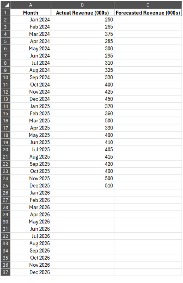
Below is a screenshot of two years of revenue data. We will use this to forecast revenue for the next 12 months based on historical data.

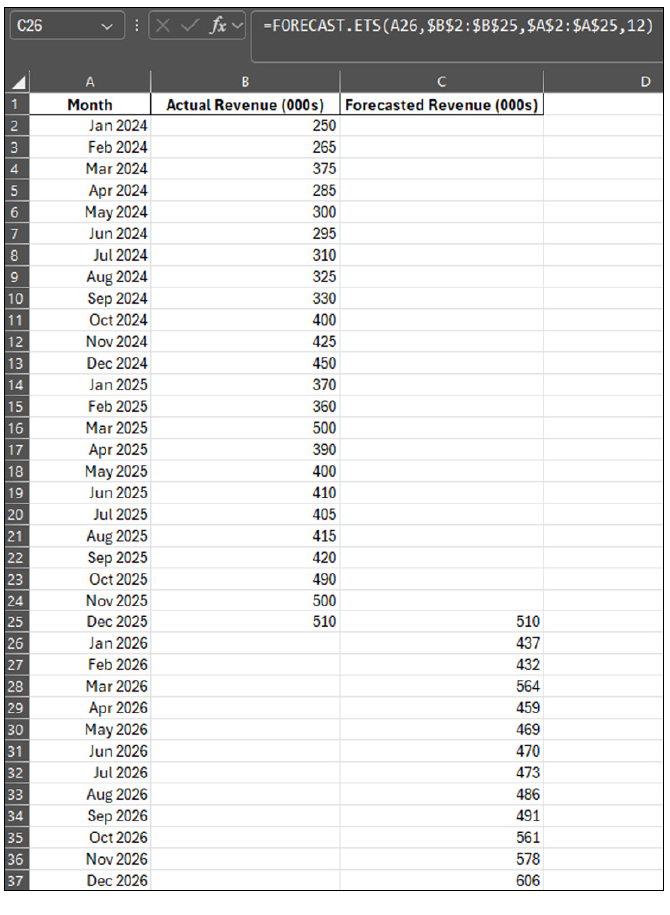
To project January through December 2026 revenue, enter the following formula in cell C26: =FORECAST.ETS(A26,$B$2:$B$25,$A$2:$A$25,12). Let’s break down this formula. The first argument, target_date, references cell A26, which is January 2026, the first month we want to forecast. The second argument, values, references our historical revenue values for 2024 and 2025. The third argument, timeline, references the corresponding dates for those historical values. Let’s also enter a value for the fourth argument, seasonality, although it is optional. The reason is that we make sure that Excel picks up on the seasonality of our rather short data period. Enter 12 because our data is annual. There is no need to enter anything for the fifth argument, data_completion, because we have no missing data. We also do not enter anything for the sixth argument, aggregation, because we do want Excel to use average, which is the default. Include absolute references ($) in arguments two and three so those ranges do not change. Drag the formula down to cell C37. Finally, enter =B25 into cell C25. The reason for this is that it will fill the gap between December 2025 and January 2026 when we chart our data. See the FORECAST.ETS formula and its results in the screenshot below.

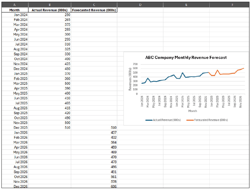
The forecasted numbers for 2026 can be visualized using a simple line chart that shows the historical data along with the forecasted data, as shown on the next page (see “10 Types of Excel Charts for Data Visualization,” JofA, Oct. 1, 2024). This simple chart makes it easy to understand the seasonality of this company’s revenues.

Alternatively, if the seasonality is left out, the line chart would reflect a linear trend for 2026, as shown in the following screenshot. (Editor’s note: Excel has two linear functions, FORECAST and FORECAST.LINEAR, that use the same syntax, but Microsoft recommends using FORECAST.LINEAR.)

Traditional forecasting methods that just have a linear line for the forecasted periods do not offer the same benefits to the user as the exponential smoothing forecasting method. Forecasting, in general, is critical for budgeting, cash flow management, performance evaluation, and resource allocation, just to name a few. FORECAST.ETS offers more accurate information to make these decisions.

About the author

Kelly L. Williams, CPA, Ph.D., MBA, is an associate professor of accounting at the Jones College of Business at Middle Tennessee State University.

Submit a question

Do you have technology questions for this column? Or, after reading an answer, do you have a better solution? Send them to jofatech@aicpa.org.