Create a dynamic to-do list with Excel’s checkboxes

Q. I currently keep a static to-do list, and I would like to update it to be more dynamic. Do you have any advice?

A. Microsoft Excel is best known for crunching numbers, but it’s also a powerful tool for organizing tasks. Checkboxes can help you create interactive to-do lists and other types of lists that track progress. They can also provide you with an interactive way to mark tasks as complete. Let’s look at a few ways to use these for our to-do list.

It’s important to note that checkboxes can be created in Excel in many ways, depending on your version. In this demonstration, I used Microsoft Excel 365 for PCs, but other versions may work differently. To follow along, you can download an Excel file with a static to-do list (you can also download a completed Excel file with checkboxes). A video demonstration of creating to-do lists using checkboxes is available at the end of this item.

The screenshot below shows the to-do list I was keeping in Excel until recently.

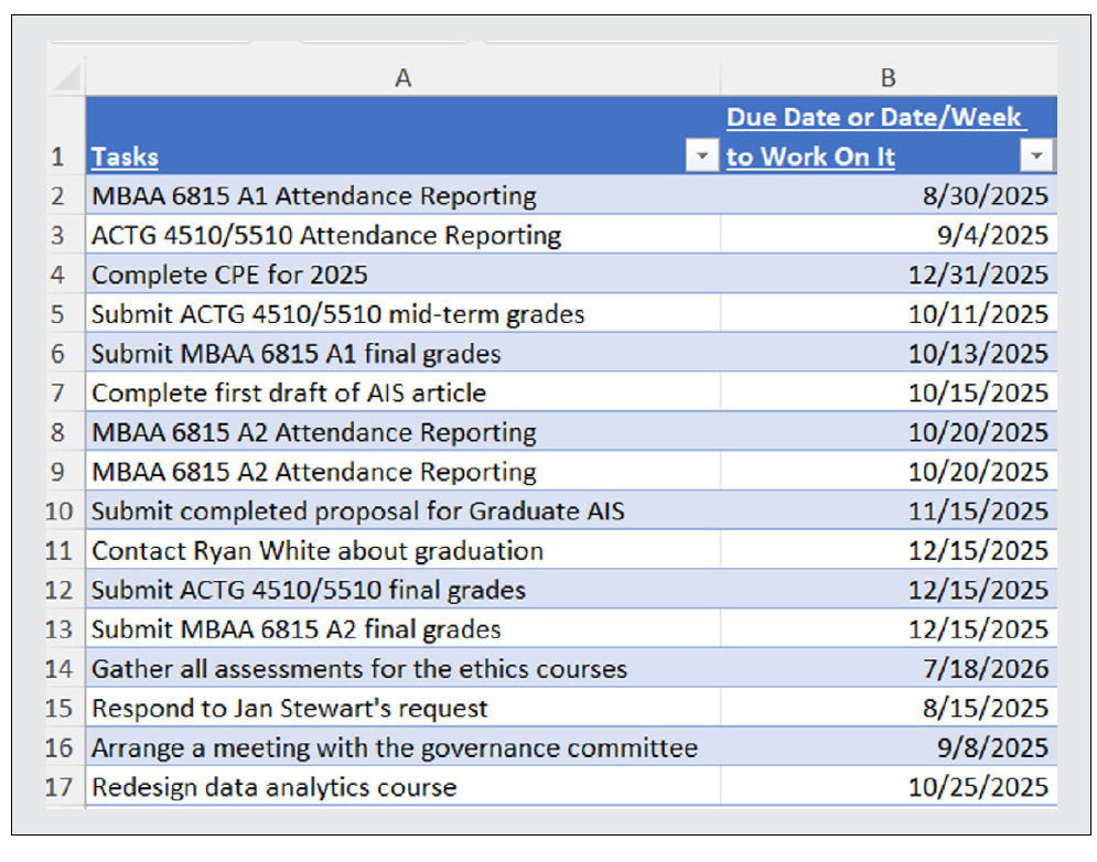
For this list, I placed the task in column A and the due date in column B. Once I completed a task, I would delete it and redo a manual sort on the due dates, so I knew what took priority. It wasn’t all bad, but I have found some more useful ways to keep my to-do list organized. Let’s go through the steps to add some improvements.

Take the old version of my Excel to-do list, add a third column to the table, and title it Completed. Select cells C2:C17, the current length of my to-do list. Don’t worry, the selection will expand or retract as the number of items changes. Go to the Insert tab on the ribbon and click Checkbox in the Controls group. As you can see below, there is now a checkbox for each item.

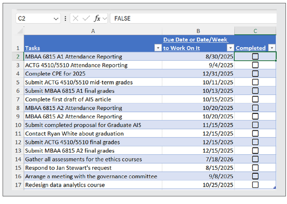
Notice the formula bar for cell C2 states FALSE. This is because the box is unchecked. Once it is checked, the formula bar will state TRUE.

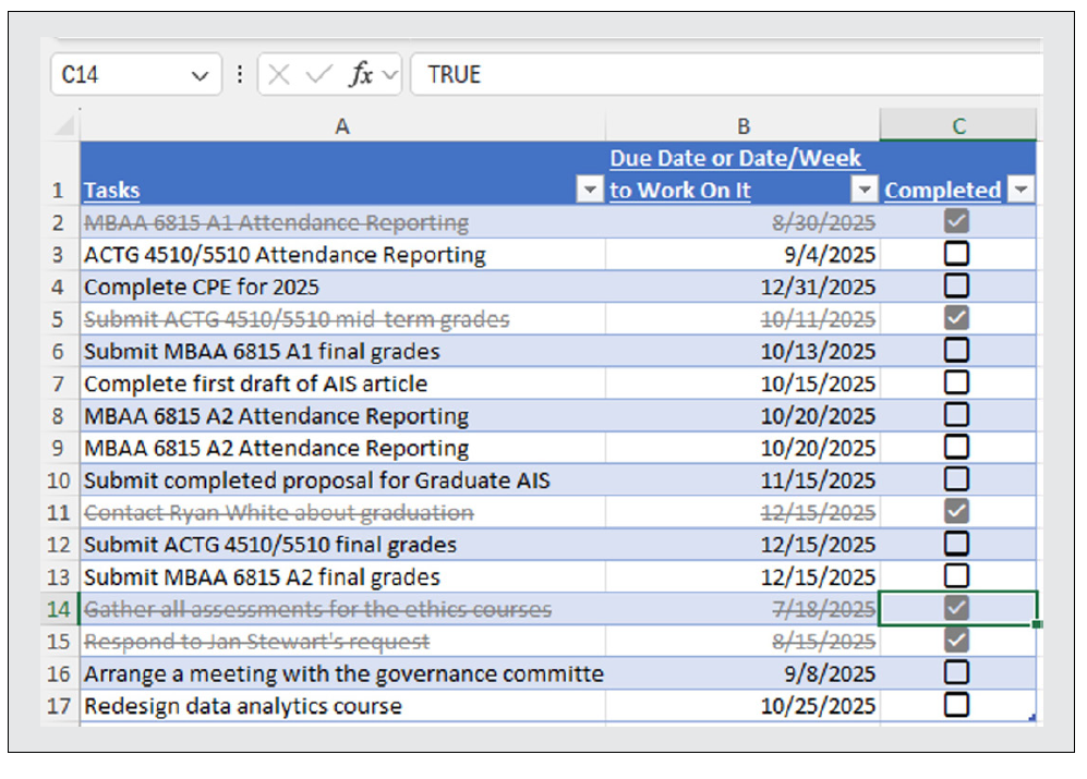
In addition to using a checkmark, I would also like to strike through completed items, so let’s add some conditional formatting. Select cells A1:C17, go to the Home tab on the ribbon, and click Conditional Formatting in the Styles group. Select New Rule and choose Use a formula to determine which cells to format. Under Format values where this formula is true:, enter =$C1. Next, click Format within that same Edit Formatting Rule window, select Strikethrough under Effects, and choose a lighter color under Color. Click Apply, then OK.

Now, all your completed items display a checkmark, a strike through that row, and a lighter color so they are less obvious than our uncompleted tasks. Also, note that in the formula bar of a checked checkbox, the formula bar displays TRUE. See the updated version of my to-do list below.

I like this, but because I prefer having my tasks sorted by due date, let’s take this a step further. Instead of using a manual sort, like I used to do, you can use an automatic sort.

Click in cell E1 and enter the formula =SORT(ToDoList,2,1). The syntax for the SORT function is =SORT(array,sort_index,sort_order,by_col). The required argument is the Array argument that defines the range or array to sort. The remaining three arguments are optional.

• Sort_index is the number of the column or row to sort by.
• Sort_order indicates the sort order:
  • 1 or omitted = Ascending
  • -1 = Descending
• By_col indicates the sort direction:
  • FALSE or omitted = Sort by row
  • TRUE = Sort by column

ToDoList is the name of the entire table, so define that as your array to sort. The sort_index should be defined as 2 because we are sorting by the second column, the due dates (column B), of the array. The sort_order is set to one to sort in ascending order. In this case, you can also leave sort_order blank, since ascending order is the default. Finally, leave by_col blank to sort by row. You can also enter FALSE to have it sort by row. Now, this formula will sort the to-do items by their due date. But we also want the completed items moved to the bottom of the list, regardless of when they were due, so let’s add another sort to this same formula.

In cell E1, modify the formula to =SORT(SORT(ToDoList,2,1),3,1). We are using the same SORT function again, and you can reference those arguments above. What we have done is start a new sort function using the sorted due dates as our array. So, we have a sorted column of due dates, then we define sort_index as 3 because we want to sort by the status of the completed items. Define the sort_order as 1 so it will be in ascending order. Remember, checked items have a value of TRUE and unchecked items have a value of FALSE. Since we want the unchecked items to appear first, we want these to be sorted in ascending order. See below to view the to-do list with checkboxes that automatically sort completed vs. uncompleted items, then sort by the due date. The formula is also listed below.

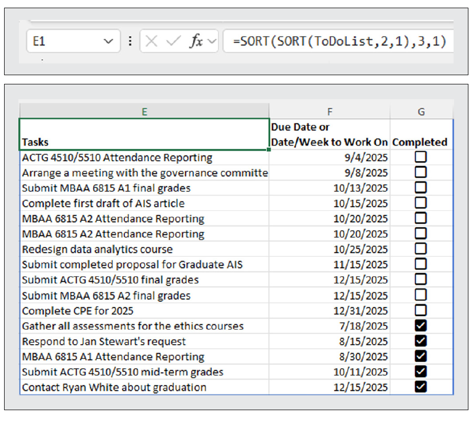
Any time you check a box as completed in the C column, the range in E:G will be updated. Similarly, anytime you add or delete an item to the to-do list in columns A–C, the range in E:G will automatically update.

One final addition I wanted to create for my to-do list is a list that contains only outstanding items and eliminates completed items. To do this, I used the FILTER function. The syntax for the FILTER function is =FILTER(array,include,if_empty), where the first two arguments are required and the third is optional. The array argument defines the range or array to filter. Next, include defines an array of Booleans (TRUE or FALSE results). The third argument is what you want returned if no items identified with Include are found.

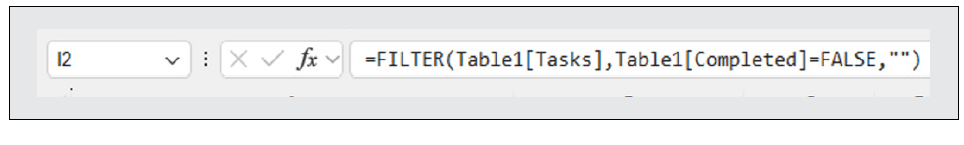
In cell I1, create a title called Tasks Remaining to Complete:. In cell I2, enter =FILTER(Table1[Tasks],Table1[Completed]=FALSE,””). The array is the tasks column (column A) in the to-do list table. The include argument is the completed column (column C) in the to-do list table that equals FALSE (meaning an unchecked box, i.e., an incomplete task). So far, this means filtering for incomplete tasks. Now, what if the task is completed? That is where the third argument comes in, if_empty. Define that argument with “” to instruct Excel not to include completed tasks at all. See below for the formula.

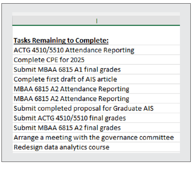
The remaining list will look similar to the one shown below, with all completed tasks eliminated from the list.

Excel checkboxes can be used for many other purposes, such as a month-end close checklist, an internal control compliance checklist, an audit preparation tracker, a tax document collection checklist, and a client onboarding checklist. The list goes on. Give them a try!

About the author

Kelly L. Williams, CPA, Ph.D., MBA, is an associate professor of
accounting at the Jones College of Business at Middle Tennessee State University.

Submit a question

Do you have technology questions for this column? Or, after reading an answer, do you have a better solution? Send them to jofatech@aicpa.org.