Using 3 Excel View tools to manage large spreadsheets
Q. I work with large spreadsheets. These spreadsheets have hundreds or even thousands of rows and often 10 or more columns. It’s so much to process that I become confused and make mistakes. Does Excel offer a way to simplify what I’m looking at so it’s not so overwhelming?
A. Microsoft Excel has features to help solve this problem. Go to the View tab on the ribbon to find these tools, which don’t modify your data but instead change your view so you can better concentrate on what matters most. Let’s look at three of these View features and then run through how to use them in an example.
Freeze Panes
When working with large datasets in Excel, it’s easy to lose track of your column headers or row labels as you scroll. That’s where the Freeze Panes feature becomes a valuable tool. Freeze Panes allows you to lock specific rows or columns in place, so they remain visible while you scroll through the rest of your worksheet.
To use this, go to View > Freeze Panes and select the dropdown arrow. You will see three options:
- Freeze Panes: Freeze both rows and columns above and to the left of the active cell.
- Freeze Top Row: Freeze only the top visible row.
- Freeze First Column: Freeze only the first visible column.
Choose the one that best suits your needs.
Focus Cell
The new Focus Cell feature is designed to help users concentrate on the most relevant portion of their workbook without distractions. Available in Excel for Microsoft 365, Focus Cell makes your spreadsheets more user-friendly, especially when working with complex or densely populated sheets.
Click on the cell where you want to focus. The focus could be an individual cell, its associated column, or row. Go to the View tab and choose Focus Cell in the Show group. The column and row surrounding the focused cell are now color-coded. You can also choose the color you want to use by clicking the dropdown arrow next to Focus Cell > Focus Cell Color and choosing the color you prefer. Note that any subsequent cell you click on will become the color-coded focus cell until you turn off the feature.
Zoom to Selection
Zoom to Selection automatically adjusts the zoom level of your worksheet, so that the selected range fills the entire visible Excel window. It eliminates the need for manually adjusting zoom percentages.
Select the cell or range of cells you want to zoom in on. Go to View and then select Zoom to Selection in the Zoom group.
A look at the 3 View tools in action
Let’s look at an example and see how easy and helpful these three features are. The screenshot below shows a snippet of a large dataset that we will use. To create these instructions, I used Microsoft Excel 365 for PCs, so other versions may work differently. To follow along, you can download an Excel file with a large dataset. A video demonstration of using these View features is available at the end of this item.
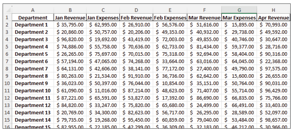
The dataset in the Excel file is so large that I could capture only a small part of it in the screenshot. Even so, I can demonstrate how easy it is to get lost in the numbers. Look at what happens when I scroll down and across.
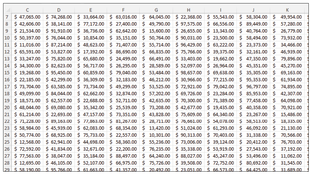
Now I can’t even see the labels for the rows and columns. This makes keeping track of the numbers you are looking for very difficult. You can fix this issue with the Freeze Panes tool. Place your cursor in cell B2 and then go to View > Window > Freeze Panes and select Freeze Panes from the three options that pop up. This tool freezes the column(s) and row(s) above and to the left of the selected cell (usually the top left data cell). After setting Freeze Panes from B2 in this example, I can scroll down or across and still see the labels, as shown below.
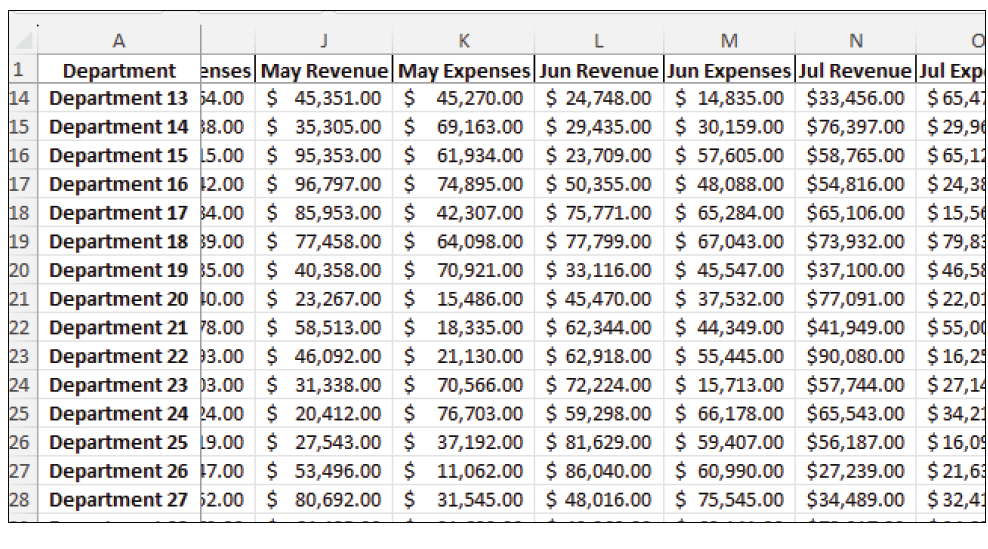
This is better, but it is still hard to keep track of what cell, column, and row you are on in large datasets. Remember, this is just a snippet of a large dataset.
Let’s use the Focus Cell feature on our dataset with frozen panes. Place your cursor in cell L23 and follow the instructions in the Focus Cell section above. See the screenshot below.
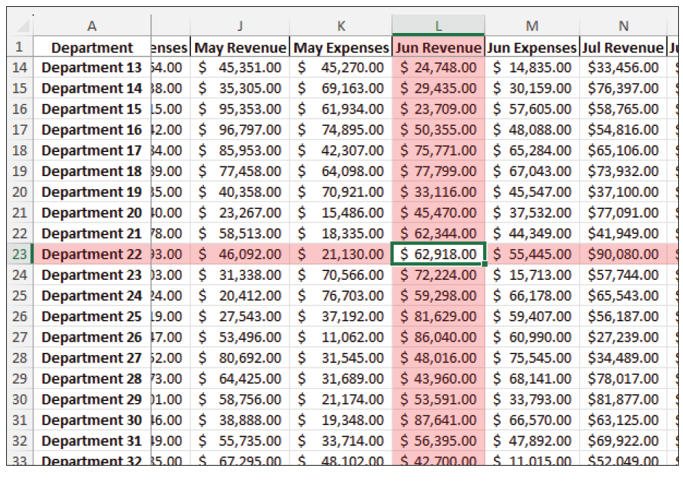
There is no mistaking that we are looking at the cell that contains June Revenue for Department 22 and the associated column and row.
Let’s explore another way to view our data — Zoom to Selection. Select cell range H13:J16 and follow the instructions in the Zoom to Selection section above. See the screenshot on the next page. This is not a snippet; this is the entire screen.
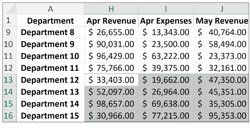
Note that because we had Freeze Panes on, Excel included our labels along with our range.
The features are simple tools to make your information in Excel more digestible, especially for professionals who deal with large or complex data. They don’t change your formulas or data; they just simplify your view.
About the author
Kelly L. Williams, CPA, Ph.D., MBA, is an associate professor of
accounting at the Jones College of Business at Middle Tennessee State University.
Submit a question
Do you have technology questions for this column? Or, after reading an answer, do you have a better solution? Send them to jofatech@aicpa.org.


