Using Excel’s TEXTBEFORE AND TEXTAFTER functions to easily tame messy data

Q. How do the TEXTBEFORE and TEXTAFTER functions in Excel work?

A. Excel’s TEXTBEFORE and TEXTAFTER functions allow users to quickly split up text in ways that used to require combinations of functions like LEFT, RIGHT, MID, and FIND, leading to some confusing formulas. Fortunately, Excel has created TEXTBEFORE and TEXTAFTER to make these tasks much simpler. If you are interested in Excel’s text functions, you can also read the August 2023 Tech Q&A article “Join Text in Excel”, which explains the function TEXTJOIN, and the previous item in this month’s Tech Q&A “Using TEXTSPLIT to Dissect Excel Text Strings”.

TEXTBEFORE function

The TEXTBEFORE function pulls what comes before a delimiter. The syntax for the TEXTBEFORE function is = TEXTBEFORE(text, delimiter, [instance_num], [match_mode], [match_end], [if_not_found]).

The required arguments are the text and delimiter arguments. The text argument references the text or cell where you’re searching. The delimiter is the marker that separates out the data you want to split.

The last four arguments are optional.

• Instance_num is the instance of the delimiter before which you want the text extracted.
  • 1 or omitted = Extracts the text before the first occurrence of the delimiter
  • -1 = Extracts after the last occurrence of the delimiter
• Match_mode controls case sensitivity.
  • 0 or omitted = Case sensitive
  • 1 = Case insensitive
• Match_end treats the end of the text as a delimiter.
  • 0 or omitted = Don’t match
  • 1 = Do match
• If_not_found is what to return if the delimiter isn’t there. By default, it returns N/A, or you can enter what to return instead.

TEXTAFTER function

The TEXTAFTER function pulls what comes after a delimiter. The syntax for TEXTAFTER is the same as TEXTBEFORE. The only difference is the purpose of Instance_num. It should now contain the instance of the delimiter after which you want the text extracted.

If you would like to follow along in using these functions, you can download this Excel workbook and view the video at the end of this item.

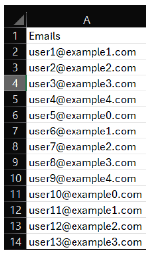
Let’s do some examples to see how these functions work. We will start with a very simple one. Let’s separate the username and the domain name from a list of emails. See below for the dataset we will use:

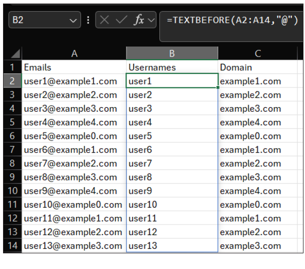
Note the delimiter here is the at symbol (@), and the username is the text that appears before that delimiter. I want my usernames in column B, so I place my cursor in B2, under the “Usernames” header, and use the TEXTBEFORE function since the username is what I want extracted. The argument for text is the list of emails, which is A2:A14 in this scenario, and the argument for delimiter is “@.” That’s it. We don’t need any of the optional arguments to do anything besides their default, so I will leave them all blank. See the screenshot below of the TEXTBEFORE function.

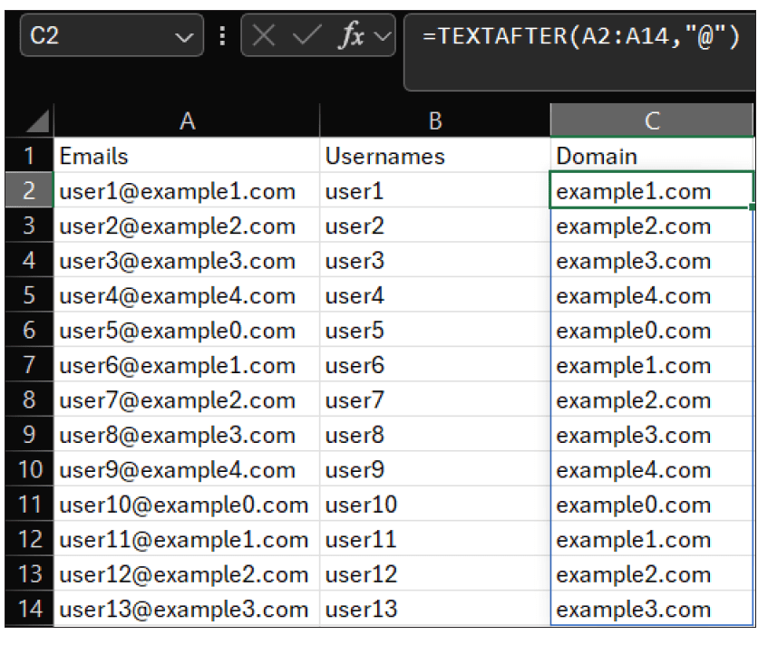
I want the domains to appear in column C, so I place my cursor in column C. Because the domains are after our delimiter, I used the TEXTAFTER function. Again, the argument for text is our list of emails, which is A2:A14 in this scenario, and the argument for delimiter is “@.” Remember, they both have the same syntax. The only difference here is that I used the TEXTAFTER function instead of the TEXTBEFORE function. See the screenshot below.

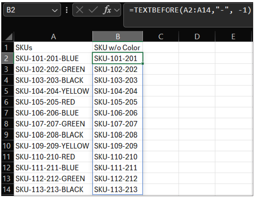
In the next example, I would like to eliminate the color found at the end of the SKU numbers in the screenshot below.

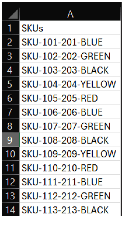
Because our delimiter is a dash (-), and there are multiple dashes in each SKU number, I have to add an extra step. I placed my cursor in cell B2, where I want the SKU numbers without color to appear. I used the TEXTBEFORE function to capture everything before that last dash. The argument for text is the list of SKU numbers, which is A2:A14 in this scenario, and the argument for delimiter is “-“. So far, it looks very similar to the first example, but if I stop the formula here, it will only extract “SKU,” which is the text before the first delimiter. This time, I need to utilize the instance_num. By default, instance num takes the first instance. This time, I need it to start reading from the end of the text string and go backward, from right to left, extracting the text from the end of the SKU until the first instance of the delimiter. In this case, that is the text that appears before the dash and color. See the formula for this in the screenshot below.

The TEXTBEFORE and TEXTAFTER functions are capable of handling many types of data and are a far easier way to extract data that does not include complex nested formulas.

About the author

Kelly L. Williams, CPA, Ph.D., MBA, is an associate professor of accounting at the Jones College of Business at Middle Tennessee State University.

Submit a question

Do you have technology questions for this column? Or, after reading an answer, do you have a better solution? Send them to jofatech@aicpa.org.