Say bye to PivotTables with Excel’s new PIVOTBY function

Q. Traditional PivotTables have always intimidated me. I see there is a new Excel function called PIVOTBY. What is the difference between it and the traditional PivotTable?

A. The PIVOTBY function in Microsoft Excel is a powerful tool designed for dynamic data analysis and summarization. It allows users to create comprehensive data summaries using a formula, offering an alternative to traditional PivotTables. With the ability to group and aggregate data along two axes, PIVOTBY provides flexibility and precision in organizing data.

Understanding how the PIVOTBY function works can significantly enhance your data analysis capabilities.

Last month, I wrote about GROUPBY, which also simplifies the traditional PivotTable. What is the difference between GROUPBY and PIVOTBY? Generally, if my groups are getting too long to analyze effectively, and I want the data to be more concise, I use PIVOTBY.

With the PIVOTBY function, you can efficiently group your data into meaningful categories, making it easier to extract valuable insights. The function’s capability to handle both row and column fields means that your data can be organized in a more structured manner than with traditional methods. Row fields are essentially the categories by which your data will be grouped horizontally. For example, if you’re analyzing sales data, you could use rows to represent different years or sales regions. Column fields are the categories that allow for vertical grouping of data. In a sales context, this might include product types or customer segments. By combining these two axes of organization, you can create a multidimensional view of your dataset, enabling a deeper analysis.

The syntax for the PIVOTBY function is =PIVOTBY(row_fields, col_fields, values, function, [field_headers], [row_total_depth], [row_sort_order], [col_total_depth], [col_sort_order], [filter_array], [relative_to]).

The following arguments are required in creating a PIVOTBY formula:

• Row_fields defines the fields to group data by rows.
• Col_fields specifies the fields to group data by columns.
• Values contains the data that will be aggregated.
• Function defines the calculation method for data aggregation. The functions you can choose are as follows:
  • SUM
  • PERCENTOF
  • AVERAGE
  • MEDIAN
  • COUNT
  • COUNTA
  • MAX
  • MIN
  • PRODUCT
  • ARRAYOFTEXT
  • CONCAT
  • STDEV.S
  • STDEV.P
  • VAR.S
  • VAR.P
  • MODE.SNGL
  • LAMBDA

The remaining arguments are optional and offer additional parameters and granularity over your data presentation:

• Field_headers, customizes column and row labels.
• Row_total_depth, determines the subtotal levels in the rows.
  • 0 or omitted = No totals
  • 1 = Grand totals only
  • 2 = Subtotals and grand totals
• Row_sort_order arranges data in ascending, descending, and custom sorting order.
• Col_total_depth determines the subtotal levels in the columns.
  • 0 or omitted = No totals
  • 1 = Grand totals only
  • 2 = Subtotals and grand totals
• Col_sort_order sorts alphabetically for text-based data, numeric sequencing for numerical values, and custom sorting.
• Filter_array allows conditional data filtering, dynamic views based on specific criteria, and multiple filter conditions simultaneously.
• Relative_to utilizes percentage calculations against totals, time-based comparisons, and multiple filter conditions simultaneously.

Currently, the PIVOTBY function is available only in Microsoft Excel 365 and Excel 2021.

If you would like to follow along in using this function, you can download this Excel workbook and view the video at the end of this article.

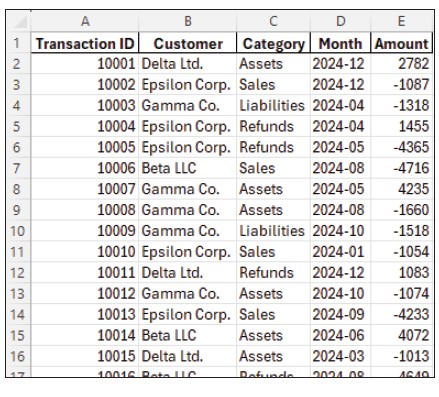
Let’s use the same dataset used in the GROUPBY article to illustrate the difference between GROUPBY and PIVOTBY and explain how to use PIVOTBY. See below for a small snippet of the spreadsheet we will use. It contains 500 transaction IDs, customers, categories, months, and amounts.

We used GROUPBY to group the transactions by customer, then by client, and calculate the total amounts. You can see the result of this below in columns G, H, and I.

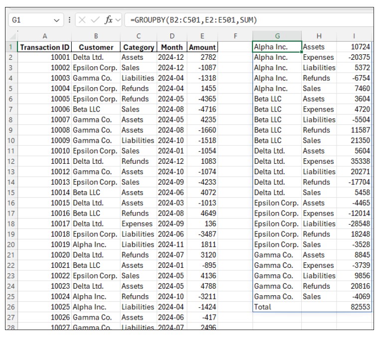
While this is very helpful, I might want this to be more concise for specific purposes or formatted differently depending on its use. That’s where PIVOTBY comes in.

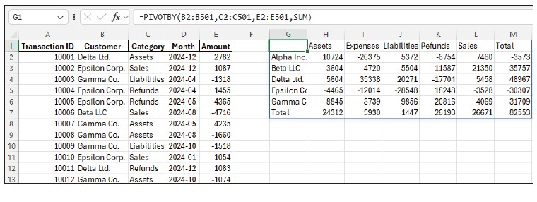
Using the same dataset, in cell G1, enter the PIVOTBY function, defining B2:B501 (all the customers) as the row_fields, C2:C501 (all the categories) as the col_fields, E2:E501 (which includes all the amounts) as the values, and SUM as the function. The formula will list each category along row 1, each customer along each row, and the total of each category shown in a table, as shown in the screenshot below.

One of the advantages of using the PIVOTBY function instead of traditional PivotTables is its ability to automatically update with new data. As your dataset changes, so do your summaries, ensuring that your analysis remains current without requiring manual intervention. Another advantage of the PIVOTBY function over traditional PivotTables is the flexibility in data analysis. You can apply custom aggregation functions using lambdas (see this article on creating lambdas, if interested).

The PIVOTBY function can turn complex datasets into easy-to-understand summaries. Give it a try!

— By Kelly L. Williams, CPA, Ph.D.

About the author

Kelly L. Williams, CPA, Ph.D., MBA, is an associate professor of accounting at the Jones College of Business at Middle Tennessee State University.

Submit a question

Do you have technology questions for this column? Or, after reading an answer, do you have a better solution? Send them to jofatech@aicpa.org.