How to use Excel’s UNIQUE Function

Q. Could you explain how the UNIQUE function works in Excel?

A. Excel’s UNIQUE is a dynamic array function that can be an essential tool for data analysts and accountants. This function allows users to extract unique values from a dataset, making it easier to identify and remove duplicates. In data analysis, removing duplicate entries is crucial for maintaining accurate and reliable datasets. This is especially important in accounting, where precise data is essential for creating financial reports and insights.

The syntax for the UNIQUE function is =UNIQUE(array, [by_col], [exactly_once]).

• Array, which is required, is the parameter that represents the range or array from which you want to extract unique values. The array can be a vertical list, a horizontal list, or a combination of both.
• By_col, which is optional, is the logical value that specifies whether the function should compare columns instead of rows. Setting this parameter to TRUE will direct the function to compare by columns, whereas FALSE (the default setting) compares by rows.
• Exactly_once, which is optional, is the logical argument that controls whether only values that appear exactly once should be returned. By default, it is set to FALSE, meaning all unique values are returned. If set to TRUE, only those unique values occurring precisely once are extracted (see the first and second screenshots below).

Note that the following content is based on Microsoft Excel 365 for PCs. Other versions of Excel may work differently.

If you would like to follow along in using this function, you can download this Excel workbook and access an accompanying video at the end of this article.

Let’s work on a few examples using the UNIQUE function. We will start with something simple but useful: identifying unique customers from a transaction log. The screenshot below is a snippet of 100 transactions, including the customers and amounts for each transaction. In cell E2, enter the UNIQUE function, defining B2:B101 (all the customers) as the array. That’s it! The formula will list each unique customer one time in a vertical list.

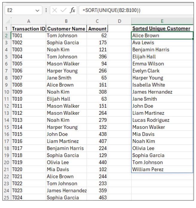
The UNIQUE function can become even more powerful when combined with other Excel functions. Let’s do an example where we will use the UNIQUE function to create a list of unique customers, as we did above, but let’s incorporate the SORT function to sort the list.

As you can see in the screenshot below, the same UNIQUE formula is entered in cell E2, including defining the same array (B2:B101). All that was to be done additionally was to add parentheses around the UNIQUE formula and include SORT in front of the UNIQUE formula.

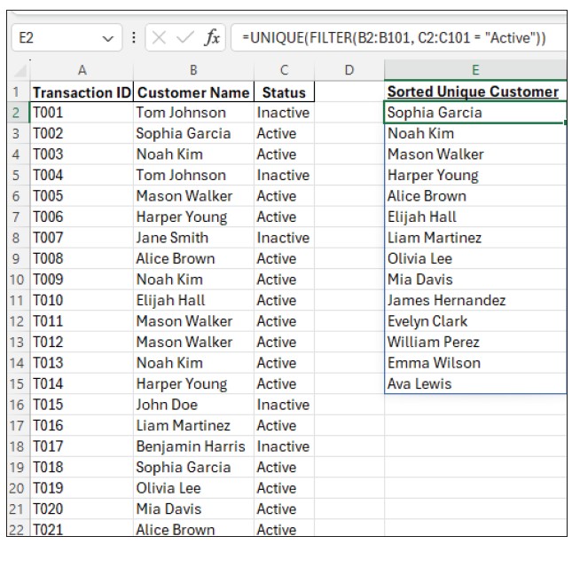
Another Excel function that pairs well with UNIQUE in the same formula is FILTER. When combined, FILTER can limit the results received from UNIQUE based on specific criteria, making it a powerful way to extract unique values that meet certain conditions. Let’s do an example where we will use the UNIQUE function to create a list of unique customers, as we did above, but let’s filter the list based on whether the customer is active.

In cell E2, again use the UNIQUE function, but this time, the array will be defined as FILTER(B2:B101, C2:C101 = “Active”). See the screenshot below for the formula and the results.

Let’s use the UNIQUE function in one more example. This time the dataset we have been using has the first and last names in different columns. We would still like to identify unique customers from the transaction log by entering my formula one time, and Excel returns the customers’ names.

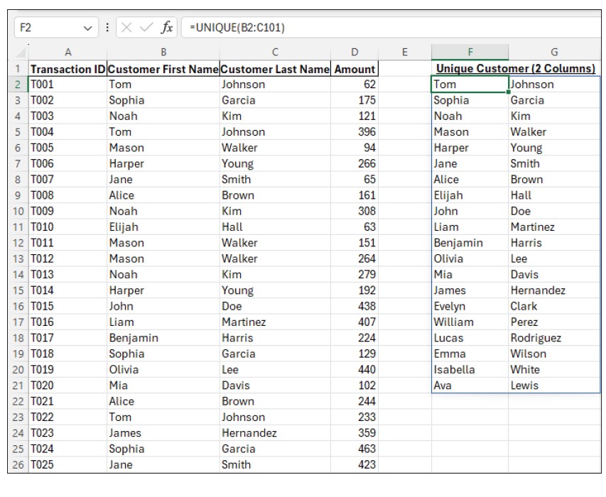
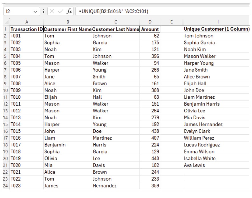
We have a couple of options on how these names are returned. One, we can have Excel return the unique list of first and last names in two columns. We still only need to create one formula for this. Two, we can instruct Excel to combine the first and last names into one cell, again with just one formula.

In the first scenario, we create a unique list of customers that pulls both the first and last names from two different columns into two different columns, and we build the formula in cell F2. Instead of the formula referencing an array that is all in one column, we will reference the array from both source columns. See the screenshot below for the formula and results.

In the second scenario, we do the same as the first scenario, but now we will extract the unique list of customers’ first and last names from two columns and have them return all in one column. Let’s build our formula in cell I2. We are still using one UNIQUE formula to pull from both columns, but this time we will use “&” to join the two columns into one. See the screenshot below for this formula and to see the first and last names be returned to one column.

About the author

 Kelly L. Williams, CPA, Ph.D., MBA, is an associate professor of accounting at the Jones College of Business at Middle Tennessee State University.

Submit a question 

Do you have technology questions for this column? Or, after reading an answer, do you have a better solution? Send them to jofatech@aicpa.org.