Change text to sentence case in Excel

Q. I read your August 2022 JofA article about changing the case of text in Excel to upper, lower, and proper, but some of my data comes in sentence form. Is there any way to convert those text strings to sentence case?

A. Excel does not have a built-in function to change a text string to sentence case, but it can be done in a few ways. There are some very simple approaches that work, such as Flash Fill, but those are not dynamic; i. e., the formatted text does not change as the data changes. You could also create code, but this can become overwhelming for some users.

Perhaps Excel will create a built-in function to convert text to sentence case in the future, but until then, a formula will work. If you would like to follow along in building this formula, you can download this Excel workbook and also access a video at the end of this article.

Note that the content that follows is based on Microsoft Excel 365 for Pcs. Other versions of Excel may work differently.

Let’s start with the actual formula, =UPPER(LEFT(T3,1))&LOWER(RIGHT(T3,LEN(T3)-1)), and then break it down and discuss each piece. If you aren’t interested in the how and just want to use the formula, that’s fine. Just copy and paste it into your spreadsheet, and it will work as long as the formula correctly references the cell that contains the text string you want converted to sentence case (T3 in the example formula above).

See the screenshot below to see the spreadsheet we will use to illustrate the formula for transforming text into sentence case. The cells in column T are in sentence form but are not consistently presented in sentence case. The spreadsheet would look much more professional with column T cleaned up. Let’s break down the formula we will use to accomplish this task.

The first part of the formula is =UPPER(LEFT(T3,1)). It capitalizes the first letter of the first word in the sentence. The LEFT function instructs Excel to go to the far left of the text string; “T3” tells Excel that the text string is in cell T3; and “1” tells Excel how many characters from the far left of the text string to extract.

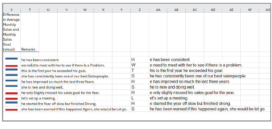
The UPPER function instructs Excel to take that first character in cell T3 and capitalize it. I inserted just this portion of the formula in cell Z3 and copied it down to cell Z12. See the screenshot below of the first letter of the first word in each sentence shown as capitalized in column Z.

The next portion of the formula is LOWER(RIGHT(T3,LEN(T3)-1)). Although we will ultimately connect the two halves of the formula, let’s explore what the second part does. The RIGHT function instructs Excel to go to the far right of the text string; “T3” tells Excel that the text string is in cell T3; and LEN tells Excel to determine how many characters are in the text string. We subtract 1 because we don’t want to include the first character. We already took care of that character with the first half of our formula. The LOWER function instructs Excel to take all the characters after the first character and make them lowercase.

I inserted just the second portion of the formula in cell AA3 and copied it down to cell AA12. (Since I inserted this second half of the formula in a new cell, I added an equal sign (=) to the beginning of the formula.) See the screenshot below of all the letters that appear after the first letter in each sentence shown as lowercase in column AA.

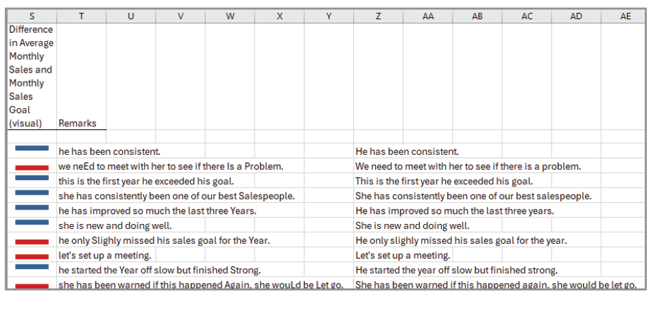
Now let’s join the first and second parts of the formula by using an ampersand (&). The formula is: =UPPER(LEFT(T3,1))&LOWER(RIGHT(T3,LEN(T3)-1)). I inserted the formula into cell Z3 and copied it down to cell Z12, then deleted the formulas in column AA. See the screenshot below for the remarks put in sentence case.

At this point, I copy my revised sentences in column Z and paste them as values in column T. The reason that I need to paste them as values is that the cells currently contain formulas. If I had pasted the formulas over the source data, the values would no longer be correct. Copy the formulas in column Z, put your cursor in cell T3, and click Home on the Ribbon. Click the drop-down arrow under Paste in the Clipboard group and select Paste Special. Choose Values in the Paste Special window and click OK. Delete the formulas in column Z. See the screenshot below for your revised, more professional-looking spreadsheet.

About the author

Kelly L. Williams, CPA, Ph.D., MBA, is an associate professor of accounting at the Jones College of Business at Middle Tennessee State University.

Submit a question

Do you have technology questions for this column? Or, after reading an answer, do you have a better solution? Send them to jofatech@aicpa.org. We regret being unable to individually answer all submitted questions.