Identify and delete duplicates in Excel

Q. What is the best way to identify duplicate transactions that could have been entered into my Excel spreadsheet?

A. Duplicates in spreadsheets can compromise data integrity, making it difficult to obtain accurate insights. In Excel, these duplicate entries can distort analysis and result in misleading conclusions.  It is crucial for accountants to identify and handle duplicates effectively to maintain the accuracy of their datasets.

Let’s look at a few ways to identify duplicates in Excel. To follow along, download this Excel workbook. A video demonstration is available at the bottom of this article.

Note that the walk-through and video were made using Microsoft Excel 365 for Pcs.  Other versions of Excel may work differently.

CONDITIONAL FORMATTING

Conditional Formatting in Excel is a powerful tool that allows users to easily spot duplicate values in their data.  It automatically highlights cells based on specific criteria, such as finding duplicates.  Accountants can use Conditional Formatting to improve data accuracy by quickly identifying and resolving redundancies. Let’s dive into a practical example using this method, as illustrated in the workbook provided.

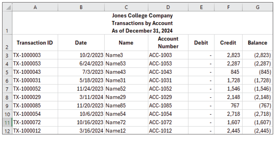
We will use a transaction report, as shown in the screenshot below.

Begin by selecting the range of cells you wish to evaluate for duplicates.  In our example, this would be column A. You can easily select the entire column by clicking on the letter A. Go to the Home tab located on the Excel ribbon at the top of your screen.  Click on Conditional Formatting.  Within the dropdown menu that appears, hover over Highlight Cell Rules to reveal additional options.  From the subsequent choices, click on Duplicate Values to focus on finding repeats in your data.

This will open a dialog box prompting you to select a preferred formatting style for highlighting duplicates. This could be a distinctive fill color or text color.  Pick the option you think will stand out best, then click OK.  Excel will instantly apply the chosen formatting to any duplicate values within your specified cell range, making them stand out.

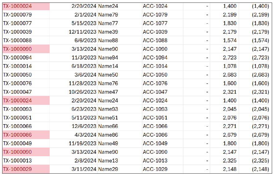
The conditional formatting clearly shows us that four transactions have been entered twice.  At this point, we can remove or deal with the duplicates however we like. See the screenshot below for a partial look at the spreadsheet with highlighted duplicates.

REMOVE DUPLICATES

The Remove Duplicates feature scans selected columns for duplicate rows based on the criteria you specify. When duplicates are found, the tool removes the extra occurrences, leaving only one instance of the data intact.

Let’s use the same transaction report as shown above to illustrate how to employ this method.

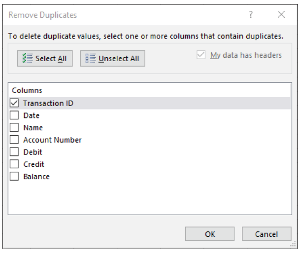
Select the range of cells or the entire table where you want to remove duplicates.  In our example, that would be just the rows that contain the transactions, A3:G50. Go to the Data tab on the ribbon and click on Remove Duplicates within the Data Tools group. In the Remove Duplicates dialog box, choose Unselect All and then click to select just the column for Transaction ID.

Click OK. A message will indicate how many duplicate values were removed and how many unique values remain.

In our example, four duplicate values were removed, and 44 unique values remain.

UNIQUE FUNCTION

UNIQUE is a Dynamic Arrays function introduced to Microsoft Excel in Office 365.  The function is designed to automatically return a list of unique values from a specified range or array. The UNIQUE function has many uses, among them identifying duplicates in Excel.

Turning back to the same transaction report, let’s walk through how to use the UNIQUE function to identify duplicates.

Select an empty cell where you want your list of unique values to appear.  For this example, chose cell I3 and you’ll easily be able to compare the results.  Using the syntax =UNIQUE(range), enter into cell I3 =UNIQUE(A3:G50) and press Enter. This will produce a spilled array that includes the 44 unique transaction Ids and their associated information. As you can see in the screenshot below, the duplicates are removed in the spilled array on the right, which has four fewer rows than the original dataset on the left (note that the column headers were added over the spilled array manually and that rows 3 through 33 were hidden to produce a screenshot of reasonable size).

Identifying and managing duplicates in Excel is a critical step for accountants aiming to maintain the
integrity of financial records. The meticulous nature of accounting work demands precision, and duplicate data can significantly hinder this requirement.

About the author

Kelly L. Williams, CPA, Ph.D., MBA, is an associate professor of accounting at the Jones College of Business at Middle Tennessee State University.

Submit a question

Do you have technology questions for this column? Or, after reading an answer, do you have a better solution? Send them to jofatech@aicpa.org.

Identify and delete duplicates in Excel
This article looks at a few ways to identify duplicates in Excel.