- column
- TECHNOLOGY Q&A
Move quickly with Excel’s Navigation Pane
Related
Differentiating agentic and generative AI — and more with a Tech Q&A author
How AI is transforming the audit — and what it means for CPAs
Promises of ‘fast and easy’ threaten SOC credibility
TOPICS
Q: Could you tell me more about the Navigation Pane in Excel?
A: The Navigation Pane in Excel is a useful tool that allows users to easily move around and manage large workbooks. It provides a way to quickly navigate to specific sheets, cells, tables, charts, or other objects within a workbook. The pane can also be used to search for specific content within a workbook, making it an efficient way to find and edit large amounts of data. You can click on a tab or even specific information within that tab from the Navigation Pane and be taken directly to it.
To open the Navigation Pane, go to the View tab and click on Navigation. The first time you do, a dialog box may appear asking if you want to try the Navigation Pane. See the screenshot below.

So, how does the Navigation Pane work? Let’s look at a workbook. To follow along, download this Excel workbook. A video demonstration is also available at the bottom of this article.
Note that the walkthrough and video were made using Microsoft Excel 365 for Pcs. Other versions of Excel may work differently.
The Navigation Pane is similar to a Table of Contents and is especially useful in a large workbook that contains a lot of data. Let’s look at the first tab in our workbook: the Dashboard (see the screenshot below). Go to View on the Ribbon and select Navigation from the Show group.

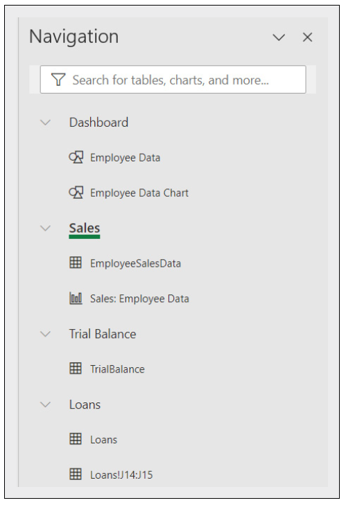
Note that the Navigation Pane lists all of the tabs in the workbook and also the data within those tabs down the right side of the screen.
You may not be satisfied with the names of your tabs or data, and you can rename them. I do not want the chart in my Dashboard tab to be called Chart 1, so I rename it. There are a couple of ways to do this. Rightclick on “Chart 1” and click Rename. Enter the name you would like. Another way to rename the chart is to click on the chart, enter the name you would like in the Name box, which is to the left of the formula bar, and click Enter. Either way, the Navigation Pane should now show the chart name, which is “Employee Data Chart”. See the screenshot below.

I would also like to clean up the title for my sales table. Because it has not been given a name, it is called the name of the tab plus the cells it populates. You can see it is called Sales!A1:A8. I use the name box to change it to “EmployeeSalesData”. Note that the name cannot have any spaces. See the screenshot below.

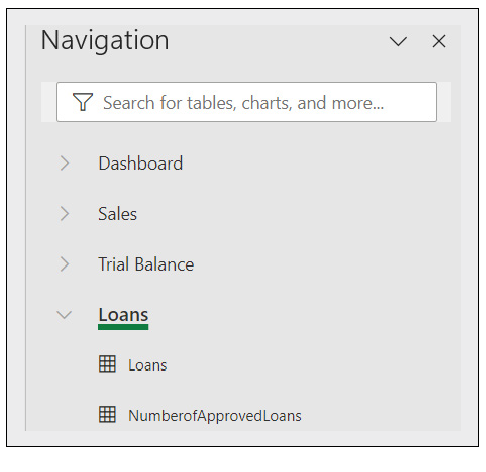
Finally, in our workbook, I would like to rename the number of approved loans appropriately on the last tab. Currently, it is just called “Loans!J14:J15”. I use the Name box to call this “NumberofApprovedLoans”. See the screenshot below.

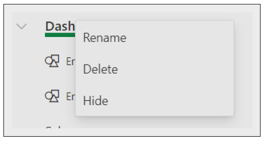
When you right-click on an item in the Navigation Pane, you get the options shown in the screenshot below. This includes the name of the tab and the content of the tabs.

You can rename an item, you can delete an item or tab, and you can also opt to hide a tab. Note that if a tab had already been hidden, that tab would have shown as light gray, and you would have had the option to Unhide.
About the author
Kelly L. Williams, CPA, Ph.D., MBA, is an associate professor of accounting at the Jones College of Business at Middle Tennessee State University.
Submit a question
Do you have technology questions for this column? Or, after reading an answer, do you have a better solution? Send them to jofatech@aicpa.org. We regret being unable to individually answer all submitted questions.


