- feature
- TECHNOLOGY
Improve audit sampling efficiency with Excel’s Solver tool
Artificial intelligence capability can significantly reduce the time and effort auditors devote to sampling estimation tasks.
Please note: This item is from our archives and was published in 2023. It is provided for historical reference. The content may be out of date and links may no longer function.

Related
AI for CPAs: From efficiency tool to decision engine
The Auditing Standards Board’s priorities for 2026 and beyond
Proposed new sustainability information AT-C sections
Stratified mean-per-unit sampling is a key tool used by auditors. The popularity of this statistical procedure arises from its unique ability to produce trustworthy confidence intervals when examining populations with low error rates. Other sampling techniques such as difference, ratio, and regression estimation yield unreliable confidence intervals unless many sample errors are detected. Given the low error rates exhibited by most accounting populations, stratified mean-per-unit sampling is the technique of choice when estimating monetary values.
Our research has identified a new method to select strata boundaries that can significantly reduce the time and effort auditors devote to sampling estimation tasks. Our findings indicate the method used to select strata boundaries is the single most important decision affecting sampling efficiency. In tests comparing conventional stratum boundary selection methods to a new method based on artificial intelligence (AI), we found that strata boundaries selected via AI yielded material improvements in sampling efficiency. Although results varied with the population examined, on average, strata boundaries selected via the new method yielded a 40% reduction in the width of confidence intervals for a given sample size. This translates into more than a 50% reduction in sample size while yielding the same confidence intervals as conventional stratum boundary selection methods.
Commercially available audit software such as IDEA and ACL are limited to conventional stratum boundary selection methods. Auditors wanting to select strata boundaries via AI must look elsewhere for this capability. Fortunately, the Microsoft Excel Solver tool has an AI capability that can be used to solve complex problems that can be used to determine stratum boundaries.
SAMPLE PLANNING WITH EXCEL’S SOLVER TOOL
In this article, we demonstrate a two-step process using the Excel Solver tool to (1) select strata boundaries and (2) determine the sample size needed to meet desired monetary precision and confidence values. A basic version of the Solver is included with Excel and can be used to find improved strata boundaries for mean-per-unit sampling applications. When using the Solver, the auditor specifies an objective formula cell to optimize by changing the values of one or more other cells. Optionally, the Solver permits specification of constraints and limitations on worksheet cell values. Once invoked, the Solver executes an intelligent search for an optimum solution. The search continues until a solution meeting all constraints and limitations is found or the auditor-specified search time limit is reached.
LOADING THE EXCEL SOLVER TOOL
Although a basic version of the Solver is included with Excel, it is not activated by Excel’s installation procedures. It must be loaded as an Add-in via the following steps:
- Select the File tab in Excel to bring up a list of menu choices in the left-most column. Click the Options selection to call up the Excel Optionsdialog box.
- In the Excel Options dialog box, select Add-ins in the left frame and verify that Excel Add-ins shows in the Manage dropdown box at the bottom of the Add-ins main area. Click the Go button to call up the Add-ins dialog box.
- In the Add-ins dialog box, check the Solver Add-in box and click the OK button.
Once the Solver is loaded, the next step is to create a placeholder calculation providing links between the objective formula cell to be optimized, other relevant cells, and the listing of population items classified into sampling strata. The links between cells must be constructed so their contents can change spontaneously as the Solver’s search process proceeds. These requirements are easily accomplished using Excel’s built-in formula functions.
CREATING A PLACEHOLDER CALCULATION
The screenshot “Initial Placeholder Calculation” presents our initial placeholder calculation. As a starting point, this worksheet employs strata boundaries selected via the equal-cumulative-square-root-of-frequency method commonly used in audit practice. Three strata are used to simplify the presentation, but any number of strata can be employed with the procedures described herein.
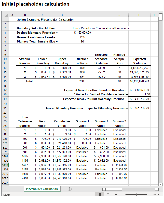
The population used in this screenshot was created for demonstration purposes as follows. First, a column vector of 2,000 cells was created with the cell contents numbered from 1 to 2,000. These numbers served as population item reference numbers. On our worksheet, this column vector begins with cell B27 and concludes with cell B2026.
Second, a recorded value for each population item was created via multiplication of the item’s reference number and a fixed multiplier. Fixed multipliers were: $1.00 for items #1 to #1,000; $2.00 for items #1001 to #1,600; and $4.00 for items #1,601 to #2,000. The result was a population of 2,000 items with a total recorded value of $4,941,900 and individual recorded values ranging from $1 to $8,000. On our worksheet, the listing of recorded values begins with cell C27 and concludes with cell C2026. Key characteristics of the population include: (1) size = 2,000 items; (2) total value = $4,941,900; (3) standard deviation = $2,558; and (4) individual values range from $1 to $8,000.
The top portion of the worksheet (rows 4–6) specifies desired monetary precision ($150,000), desired confidence level (95%), and an initial value for planned total sample size (60). The Solver needs these auditor-specified values to compute expected monetary precision (cell H19) as the search for optimum strata boundaries proceeds. The initial value for planned total sample size is not critical because optimum strata boundaries are not very sensitive to this value. However, at a minimum, the value should equal the number of sampling strata multiplied by the auditor-specified minimum stratum sample size. We presume a minimum stratum sample size of n = 20, and hence set the initial total sample size at n = 60 (20 items per stratum × 3 strata). After determining appropriate strata boundaries in step one, the value of desired monetary precision is used by the Solver in step two as the search for an optimum total sample size is conducted.
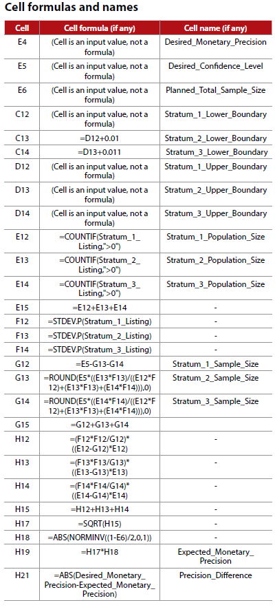
The central portion of the worksheet (rows 12–21) specifies strata boundaries, reports the resulting number of strata items and strata standard deviations, specifies strata sample sizes based on optimal allocation of the total sample, computes strata contributions to the estimator variance, and projects expected monetary precision. In addition, the deviation between desired precision and expected precision (cell H21) is computed. To ensure the reader can reproduce this worksheet, the table “Cell Formulas and Names,” below, provides a listing of all cell formulas and related names assigned to cells.
The lower portion of our worksheet (rows 27–2026) lists population item reference numbers (column B), item recorded values (column C), and cumulative population values (column D), and classifies population items into one of three strata column vectors (column E, F, or G), based on the strata boundary values specified in the worksheet range C12:D14. Note that stratum listings are all column vectors of the same length (2,000 cells).
In each stratum column vector, some cells contain numeric values (for stratum members), and other cells contain text values (for stratum nonmembers). This arrangement ensures that only valid stratum members are included when Excel computes the number of stratum items and the standard deviation of their recorded values. Also, note that many worksheet rows are hidden in the lower portion of the screenshot “Initial Placeholder Calculation” due to space limitations.
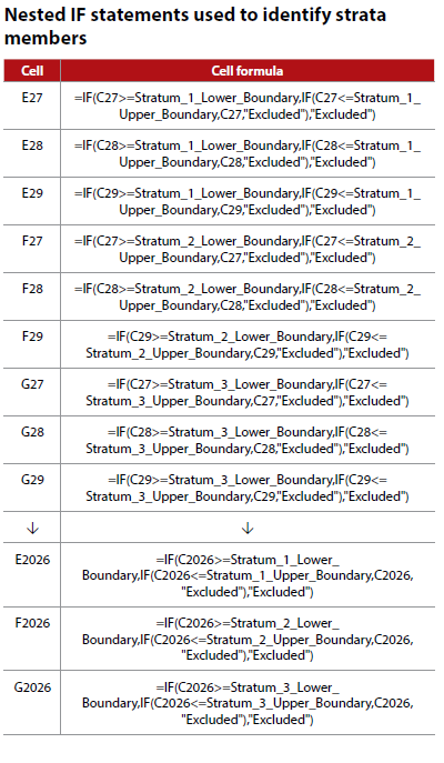
Given the need to revise stratum membership decisions spontaneously as the Solver’s search proceeds, nested IF statements are applied to the column vector containing population item values (column C). These nested IF statements compare item recorded values (worksheet range C27:C2026) to lower and upper strata boundary values (worksheet range C12:D14). When an IF statement identifies a population item as a stratum member, the IF statement places the item’s recorded value in the listing of values for that stratum, otherwise the text “Excluded” is placed in the listing for that stratum. Examples of the IF statements used to determine stratum membership are given in the table “Nested IF Statements Used to Identify Strata Members,” below.
CALLING THE SOLVER TOOL AND ENTERING INFORMATION
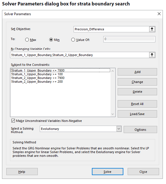
To call the Solver, select the Data tab and then select the Solver option (at the far right). When the Solver Parameters dialog box appears, the Solver must be told to minimize the difference between desired and expected precision. To do this, insert the objective formula cell reference (H21) or cell name (Precision_Difference) into the Set Objective input area and select the Min (minimize) radio button. Next, tell the Solver to vary the upper boundaries of stratum 1 and stratum 2 to change the objective formula cell value (H21 or the name Precision_Difference). This is accomplished by inserting the cell references for the upper boundaries (D12 and D13) or the related cell names (Stratum_1_Upper_Boundary and Stratum_2_Upper_Boundary) into the By Changing Variable Cells input area.
To ensure an efficient search, the Solver requires specification of lower and upper limits for each variable specified in the By Changing Variable Cells input area. To enter these limits, click the Add button in the Subject to the Constraints input area to bring up the Add Constraint dialog box. Then, for each variable listed in the By Changing Variable Cells input area, specify a lower limit and an upper limit. With two manipulated strata boundaries and two limits for each boundary, this requires a total of four constraints. In our worksheet, since individual population items range in value from $1 to $8,000, limits on strata boundaries are specified as (1) $100 and $7,800 for the stratum 1 upper boundary and (2) $200 and $7,900 for the stratum 2 upper boundary. These limits are a matter of judgment but should provide a reasonably wide search field for the Solver. If the search field is too narrow, the Solver may be unable to locate an optimum solution. Because all numeric values in a sampling application must be non-negative, a check mark should be entered in the Make Unconstrained Variables Non-Negative check box.
Finally, a solving method must be chosen from among the methods listed in the Select a Solving Method dropdown box. The methods available are Simplex LP, GRG Nonlinear, and Evolutionary. For the complex problem of selecting strata boundaries, the Evolutionary method must be selected. Once entries in the Solver Parameters dialog box are completed (see the screenshot “Solver Parameters Dialog Box for Strata Boundary Search,” below), click the Solve button to begin the search for strata boundaries.
In our application, after about 10 seconds of searching, the Solver recommends a stratum 1 upper boundary of $1,526.52 and a stratum 2 upper boundary of $3,292.76 (see the screenshot “Solver Strata Boundary Search Solution,” below).

A comparison of expected monetary precision for the equal-cumulative-square-root-of-frequency method ($411,736.28 in the “Initial Placeholder Calculation” screenshot) and expected monetary precision for the Solver Search ($169,712.65 in the “Solver Strata Boundary Search Solution” screenshot) confirm the Solver’s recommended strata boundaries yield better expected precision. Given the initial total sample size of n = 60, neither solution meets the auditor’s desired precision value of $150,000, but strata boundaries recommended by the Solver are much closer to the desired result than those provided by the equal-cumulative-square-root-of-frequency method. As a final step in this application, the Solver can be used to find the total sample size needed to meet the auditor’s desired monetary precision value.
REVISING SOLVER INPUTS TO SEARCH FOR TOTAL SAMPLE SIZE
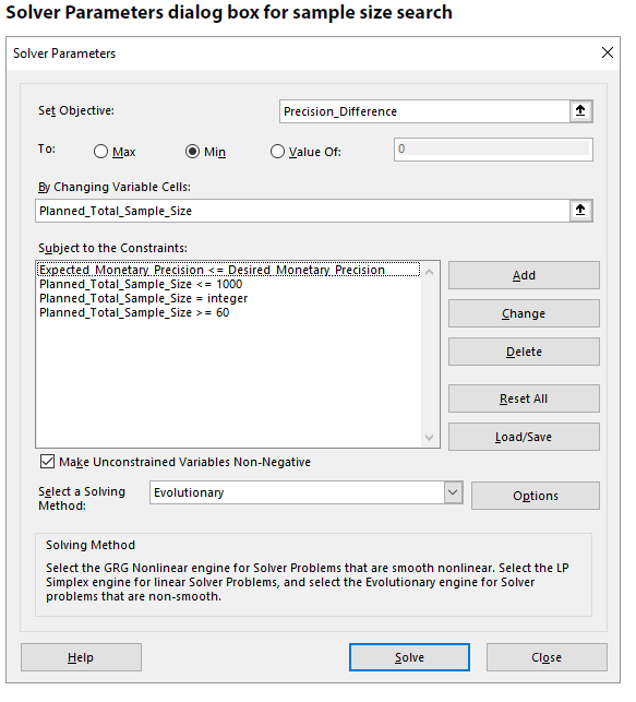
Once strata boundaries are determined, information entered into the Solver Parameters dialog box must be revised to support a search for the total sample size needed to meet the auditor’s desired precision value. To recall the Solver, select the Data tab and select the Solver option (at the far right). When the Solver Parameters dialog box appears, leave the value specified in the Set Objective input area (H21 or the name Precision_ Difference) unchanged. Also retain the: (1) radio button selection of Min; (2) check mark entered into the Make Unconstrained Variables Non-Negative check box; and (3) the Evolutionary solving method in the Select a Solving Method dropdown box.
However, the Solver must be told to vary the application sample size to change the difference between desired monetary precision and expected monetary precision (cell H21 or the name Precision_Difference). This is accomplished by replacing references to strata boundaries in the By Changing Variable Cells input area with the cell reference (E6) or cell name (Planned_Total_Sample_Size) for the application total sample size. At the same time, the lower and upper limits on strata boundaries should be removed from the Subject to the Constraints input area by selecting each constraint and using the Delete button.
To ensure an efficient search process, the auditor must specify upper and lower limits on the total sample size. To do this, click the Add button to bring up the Add Constraint dialog box. Then add constraints for an upper limit and a lower limit. In our worksheet, we specified a sample size upper limit of n = 1,000 and a lower limit of n = 60. These limits are a matter of judgment but should be specified so the Solver has a reasonably wide search field. Finally, two additional constraints must be added: (1) The total sample size variable (cell E6 or Planned_Total_Sample_Size) must be constrained to be an integer, and (2) the Solver must be told to ensure that the expected monetary precision (cell H19 or the name Expected_Monetary_Precision) is less than or equal to the desired monetary precision (cell E5 or the name Desired_Monetary_Precision).
Once the Solver Parameters dialog box entries are revised (see the screenshot “Solver Parameters Dialog Box for Sample Size Search,” below), click the Solve button to begin the search for the total sample size.
In our application, after about 90 seconds of searching, the Solver recommends a total sample size of n = 77, distributed as follows: n = 33 for stratum 1; n = 23 for stratum 2; and n = 21 for stratum 3 (see the screenshot “Solver Sample Size Search Solution,” below). Note that these strata sample sizes meet our requirement of 20 sample items per stratum. If the minimum stratum sample size requirement is not met, the Subject to the Constraints input area can be modified to specify a minimum sample size in each stratum.

The screenshot “Solver Sample Size Search Solution” indicates the Solver’s recommended total sample size is expected to provide a monetary precision of $149,114.83 and thus satisfy the desired monetary precision of $150,000. By comparison, a total sample size of n = 345 would be required to meet the desired precision objective if the equal-cumulative-square-root-of-frequency method was used. Hence, in this hypothetical application, reliance on the Solver’s recommended strata boundaries reduced the required total sample size by over 75%. For many real-world populations, we expect that strata boundaries selected via AI will yield sample size reductions of 50% or more. Given this fact, all auditors should be aware of the Solver’s capabilities. (See the sidebar, “Solver Options,” at the end of this article, about the tool’s settings.)
USING THE SOLVER WITH NONSTATISTICAL SAMPLES
The statistical formulas used in this article apply only when strata samples are chosen via random selection. However, the need to efficiently allocate audit effort exists regardless of whether the auditor selects samples randomly or via nonstatistical methods. In circumstances where the auditor plans to stratify a population and select sample items via nonstatistical procedures, using the Excel Solver to select strata boundaries will likely improve audit sampling efficiency.
Solver options
Excel’s Solver tool has many settings that affect the search process. Normally, it is not necessary to change these settings from their default values. However, if desired, the auditor can change one or more settings by selecting the Options button on the Solver Parameters dialog box. Information about Solver options is available on the web by clicking here.
If an application has a very large population or uses many strata, it may be necessary for the auditor to increase the maximum search time setting. This setting is located near the bottom of the All Methods tab of the Options dialog box. One final point: Circumstances may arise where the basic Solver tool included with Excel lacks the power or capacity to meet the auditor’s need. If this problem occurs, the auditor can purchase a more powerful add-in version of the Solver from Frontline Systems Inc.
About the authors
Thomas W. Hall, CPA, Ph.D., is a professor in the Department of Accounting at the University of Texas, Arlington; Lucas A. Hoogduin is an audit professional at KPMG Netherlands and is based in Amsterdam; and Bethane Jo Pierce, Ph.D., is an associate professor in the Department of Accounting at the University of Texas, Arlington.To comment on this article or to suggest an idea for another article, contact Courtney Vien at Courtney.Vien@aicpa-cima.com.
LEARNING RESOURCES
Advanced Excel: Practical Applications for Accounting Professionals
Written by a CPA and Excel expert, this self-study course will help you be more efficient and productive. This course covers topics including advanced PivotTables, external data ranges (ODBC), and visual basic (macros and user-defined functions).
CPE SELF-STUDY
Excel — Advanced Financial and Statistical Calculations
In this webcast, you will learn some powerful functions in Excel that will take your calculating power to the next level.
WEBCAST
For more information or to make a purchase, go to aicpa.org/cpe-learning or call the Institute at 888-777-7077.
AICPA RESOURCES
Articles
“Embracing Technology in the Audit,” JofA, Feb. 2022
“6 Lessons From Audit Experts Who Adopted AI Early,” JofA, Nov. 23, 2021
“Journal-Entry Testing Using Excel,” JofA, Nov. 2021
“More Businesses Using AI as Tools Emerge,” JofA, Feb. 24, 2020


