- feature
- TECHNOLOGY WORKSHOP
How to boost Excel efficiency with Power Query
Microsoft tool makes ongoing data mining of general ledgers much easier.
Please note: This item is from our archives and was published in 2017. It is provided for historical reference. The content may be out of date and links may no longer function.

Related
People skills: You are a human being, not a human doing
Use Excel to automate financial statement analysis
5 human competencies CPAs need in the AI age
The January 2017 JofA article “Data Mining Your General Ledger With Excel” presents a step-by-step, formula-based approach to extracting general ledger data and then scrubbing them so that they can be readily analyzed through the use of PivotTables.
The approach works very well for most analyses. Challenges occur when subsequent data are added to the general ledger, because it is time-consuming to repeat all the steps in the scrubbing process.
This article describes how Microsoft Power Query for Excel can be used to easily transform data and be applied in subsequent periods so that very little additional work has to be done to obtain clean data. While it is a best practice to do as much data scrubbing and transforming in a native application, Power Query can still add value in cleaning raw data and modeling them in a fashion that facilitates further analysis.
Power Query is a powerful tool for modeling and shaping data. While it can load data from a variety of data sources, such as Excel, comma-separated value (CSV), and text files, and SQL, MySQL, and Oracle server databases, this article focuses on loading data from a CSV or Excel file. Power Query uses an Excel spreadsheet-like interface, so navigating its features becomes second nature to an experienced Excel user.
A good way to think about when and why to use Power Query is to consider its relationship to PivotTables. While analysis is best done in PivotTables, Power Query cleans the data for best use by PivotTables.
Power Query is available in Excel 2010 and Excel 2013 as a free add-in downloadable from Microsoft’s website at microsoft.com. In Excel 2016, it is included under the Data tab in the Get & Transform group. While this article uses Excel 2016, the steps are similar in Excel 2010 and 2013.
We will use the same Excel file that was used in the above-referenced article to demonstrate how Power Query works and illustrate its added functionality in more complex situations. Download the file via the January article or by clicking here. Although the instructions in this article are geared toward QuickBooks, they can be adapted to other accounting systems.
Experienced data analysts use a standard approach to data mining. They begin with a process called ETL, which stands for extract, transform, and load. This article describes the best way to extract data from a desktop version of QuickBooks and use Microsoft Excel’s Power Query feature to transform the data so that they can be analyzed through an Excel table or PivotTable.
EXTRACTING THE FILE
Data can be exported from desktop versions of QuickBooks to Excel as either a CSV file or as an Excel file. The online version of QuickBooks exports data only as an Excel file. In either case, it is a best practice to first configure as much of the data as possible in their native application before exporting them to Excel. In QuickBooks, this is done in two steps. The first step is to choose the columns that you want included in the report. The second step involves using the Advanced… option in the Send Report to Excel dialog box to configure the file’s format.
I prefer to use a CSV file because it offers two important advantages over an Excel file. The first is that the file loads in seconds. An Excel file that contains many rows and formulas will take a very long time to fully load. The second advantage is that a CSV file writes all amounts as values, so no conversion of formulas is needed.
Begin the report configuration process by choosing the columns to be included in the report. Columns are chosen by clicking on the Customize Report button in the QuickBooks report button bar. This will open a dialog box, as shown in the screenshot “Modify Report: Reconciliation Detail.”
Modify report: Reconciliation detail
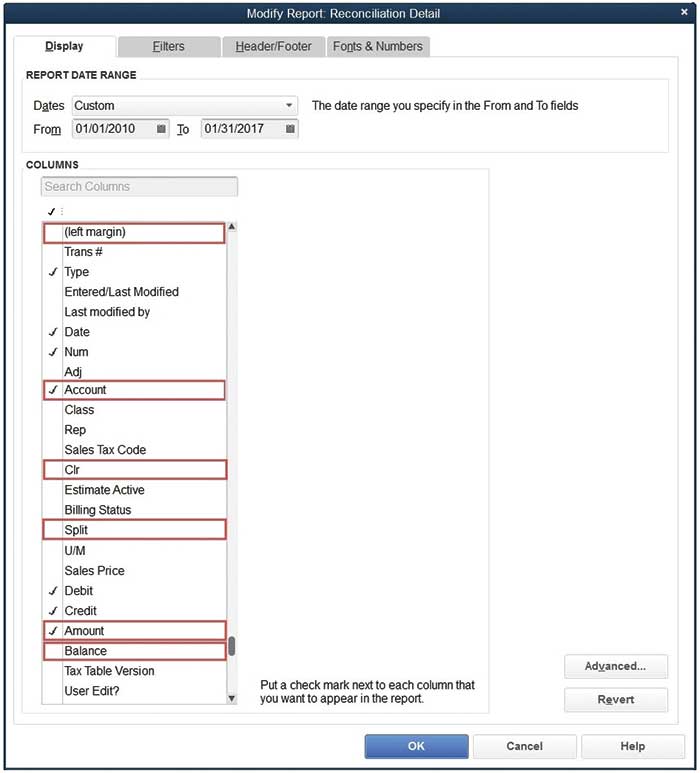
On a general ledger report, I recommend that on the Display tab you uncheck (left margin), Clr, Split, and Balance, and check Account and Amount. I suggest checking Account so that QuickBooks will write the account title in a separate column and Amount to produce a single column with all transactions.
When working with an Excel file, I also suggest that all of the QuickBooks Options in the Advanced Excel Options dialog box be unchecked as shown in the screenshot “Advanced Excel Options.” I especially recommend that the Space between columns be unchecked so that they do not have to be removed later as part of the data-scrubbing process. We will be working with an Excel file that has not been formatted in the suggested manner. This allows us to look at certain features of Power Query.
Advanced Excel options

TRANSFORMING THE FILE
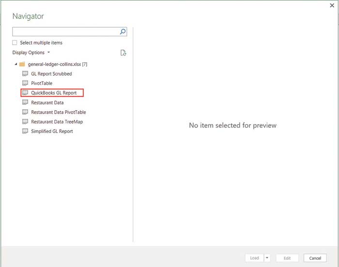
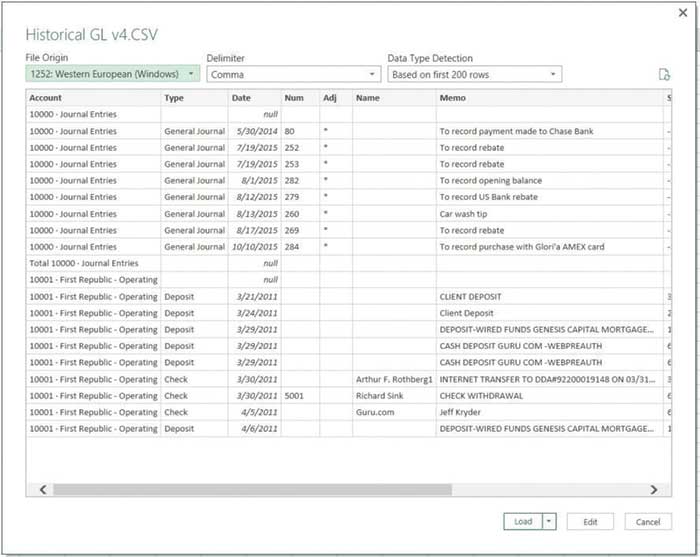
Transforming the file begins with opening a blank workbook. In Excel 2016, Power Query is accessed by clicking on the Data tab and then clicking on the drop-down arrow next to New Query in the Get & Transform group and then selecting From File. If you’re loading an Excel file, choose the top option, From Workbook. If you’re loading a CSV file, choose the second option, From CSV. When you open your Excel file in Power Query, you are presented with the Power Query Navigator dialog box, as shown in the screenshot “Navigator Dialog Box.” The navigator lists all of the worksheets within the workbook file. You’ll want the downloaded data from the QuickBooks general ledger, so pick the third item, QuickBooks GL Report, and click Edit. If you are opening a CSV file or an Excel file with only one worksheet, the navigator screen will not appear. Power Query will open a preview screen, as shown in the screenshot “Navigator Dialog Box With Preview Screen.” Click the Edit box at the bottom of the screen to load the file into Power Query’s Query Editor.
Navigator dialog box
Navigator dialog box with preview screen
The Query Editor has five tabs: File, Home, Transform, Add Column, and View. The file opens at the Home tab, where we’ll begin the transformation process. In those cases where there is no column heading in the original file, the column headings will read Column1, Column2, etc., and the actual column headings will show in the first row of the spreadsheet. In other cases, in which each column has a heading, the actual imported column headings will show as column headings.
Step 1: Click on the drop-down arrow next to Use First Row as Headers in the Transform group in the Home tab, and choose the first option: Use First Row as Headers. This will move the actual headers to the column headings area, as shown in the screenshot “QuickBooks GL Report.”
QuickBooks GL report
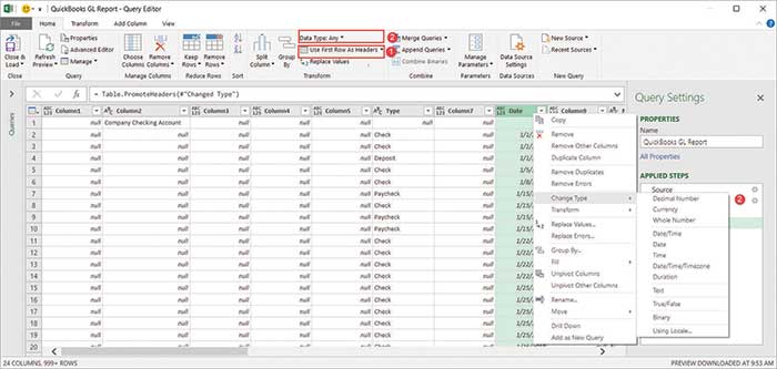
Step 2: Change the Data Type for certain columns, as shown in the screenshot “QuickBooks GL Report.” Notice that Power Query assigned an Any or a Text value to all columns as a default. Change the Date column to Date type, change the Num column to Whole Number type, and change the Debit, Credit, and Balance columns to the Decimal Number data type. Multiple columns can be accessed by either holding down the Ctrl key and clicking on each column, or adjacent columns can be accessed by clicking on the first column and holding down the Shift key while clicking on the last column in the range.
Step 3: As shown in the screenshot “Replacing Column Headings,” add the column heading “Account” to replace “Column2” by either (1) right-clicking on the column heading and choosing Rename or (2) clicking on the column heading and then clicking on the Transform tab and selecting Rename in the Any Column group.
Replacing column headings
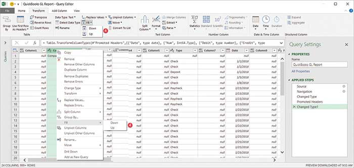
Step 4: In this step, we begin to shape the data by filling in the blank cells beneath each account title in the newly named Account column. Either right-click the Account column and choose Fill, then Down, or in the Any Column group in the Transform tab, click on Fill, then Down to replace the null entry with the account title for each account, as shown in the screenshot “Replacing Null Entries.”
Replacing null entries
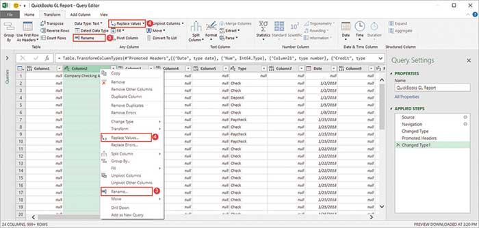
In the event that the cells under an account title are blank, they must be filled with a null entry. Again, either right-click on the column header and choose Replace Values, as shown in the screenshot “Replacing Values,” or after clicking on the column header, choose the Transform tab and then click on Replace Values in the Any Column group. Doing this will bring up the Replace Values dialog box. Leave the Value To Find box empty and enter null in the Replace With box, then click OK to close the dialog box, and automatically enter the word null in each blank cell.
Replacing values

Step 5: Remove any unwanted columns, such as Clr, Split, and Balance by selecting them and either right-clicking the column heading and selecting Remove or, after selecting a column, clicking on Remove Columns in the Columns group under the Home tab. Alternatively, you can select the columns that you want to keep and choose Remove Other Columns under the right-click menu or under the Remove Columns button.
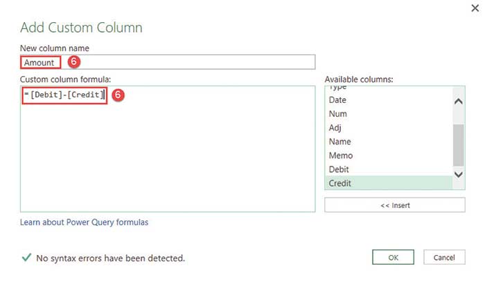
Step 6: Although the query can now be used as is, I like to show my debits and credits in one column so that I can easily see an account’s balance. To do this, begin by selecting the Debit and Credit columns and replacing the null values with a zero (0) using similar steps to those described in Step 4. Then add a new column by clicking on Custom Column in the General group under the Add Column tab. This opens an Add Custom Column dialog box, as shown in the screenshot “Adding Custom Columns.” Change “Custom” in the New column name box to “Amount.” In the Custom column formula field enter Debit — Credit by scrolling down in the Available columns box and double-clicking on Debit, entering a minus sign, and then double-clicking on Credit. The resulting formula will be [Debit]-[Credit]. Click OK to close the dialog box and generate the new column. The new column will become the right-most column in the query but can be moved by selecting it and then dragging it to your desired position. Change the data type to Decimal Number by following the steps described above.
Adding custom columns
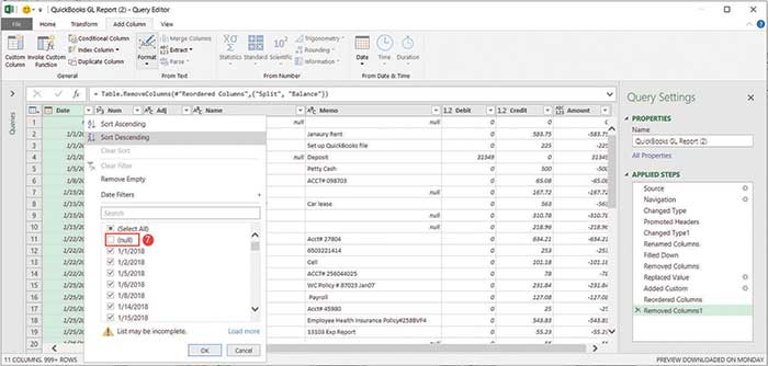
Step 7: Certain rows exported from QuickBooks either contain cell entries that we do not need or have no relevant data, such as the “account title” rows that only have the title in the Account column and the “total” rows. Notice that the Date column has a date in only those rows that have data that we want to keep. Therefore, we’ll filter this column by unchecking null, as shown in the screenshot “Removing Unnecessary Rows.” This will remove the unnecessary rows and leave us with only clean data.
Removing unnecessary rows
Step 8: Close and load the query by clicking on Close & Load in the Close group of the Home tab. This will open the shaped data in an Excel table from which you can generate a PivotTable or simply use the drop-down filter at the top of each column to filter for the results that you want.
Two major advantages of using Power Query, compared to traditional data scrubbing of files using a formula approach, are that the query does not affect your original file, as it only reads the file and does not write to it, and that it can be reused in subsequent periods with little or no additional work. Simply save the updated data with the same format and the same name as the original file. The next time you want to run the query, open the file that contains it, right-click on the query’s name in the right-hand navigation pane, and click Edit, then click on the drop-down arrow next to Refresh Preview in the Query group, choose Refresh All, and then click on Close & Load. The updated data will be added to your Excel Table.
If the query does not show, click on Show Queries in the Get & Transform group of the Data tab to open the navigator pane. Similarly, modify an existing query by right-clicking on it and choosing Edit. If you make an error when performing a step, simply click on the “X” that is in front of the incorrect step to delete it.
BROAD RANGE OF FEATURES
This article touches on a small number of the many features available in Power Query. I suggest that you investigate how Power Query can be used to simplify other tasks that were formerly done with VLOOKUP and other formulas.
Power Query’s many capabilities
This article touches only on a limited explanation of Power Query’s capabilities. Additional capabilities include the ability to parse text, merge or append files, and apply formulas to selected columns of data. Its ability to join data, another term for data matching, allows it to substitute for more complex VLOOKUP or INDEX and MATCH formulas. These capabilities will be addressed in future articles as the JofA further explores this powerful tool.
About the author
Arthur F. Rothberg (arthur.rothberg@cfoedge.com) is the founder and managing director of CFO Edge LLC, a Southern California CFO services firm that helps executives move pressing financial challenges to resolutions and clear value.
To comment on this article or to suggest an idea for another article, contact Jeff Drew, senior editor, at Jeff.Drew@aicpa–cima.com or 919–402–4056.
AICPA resources
Article
- “Data Mining Your General Ledger With Excel,” JofA, Jan. 2017
CPE self-study
- Advanced Excel: Practical Applications for Accounting Professionals (#745757, text; #163142, online access; #GT-EXPF, group pricing)
Conferences
- Digital CPA Conference, Dec. 4—6, San Francisco
- Practitioners Symposium and Tech+ Conference at AICPA ENGAGE, June 11—14, Las Vegas
For more information or to make a purchase or register, go to aicpastore.com or call the Institute at 888-777-7077.
Information Management and Technology Assurance (IMTA) Section and CITP credential
The Information Management and Technology Assurance (IMTA) division serves members of the IMTA Membership Section, CPAs who hold the Certified Information Technology Professional (CITP) credential, other AICPA members, and accounting professionals who want to maximize information technology to provide information management and/or technology assurance services to meet their clients’ or organization’s operational, compliance, and assurance needs. To learn about the IMTA division, visit aicpa.org/IMTA. Information about the CITP credential is available at aicpa.org/CITP.


